
Place names in UK and Ireland are very much influenced by their surroundings, with endings such as -hill, -ford, and -wood quite clearly referencing local geography. This post describes the creation of an interactive map that allows you to explore UK place name endings. The creation of this map involved using a number of the new D3 command line tools for manipulating geographic data, which allow the creation of optimised datasets that improve performance.
If you’re not so interested in the tech, here’s an overview of the results:
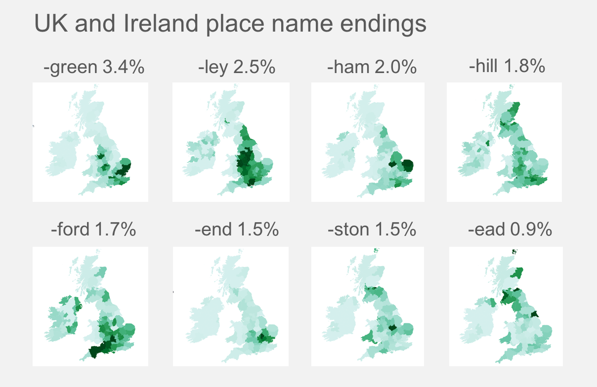
The most popular place name ending is -green, which is highly concentrated around Essex, whereas the ending -end is quite prevalent within London.
You can also explore the data in interactive form.
Introduction
I’ve been using D3 for a number of years now, but always for charts, lots of charts. Lots and lots of charts. I’ve been looking for an excuse to try out the various mapping capabilities of D3, but until recently haven’t found a good excuse.
I grew up in East Anglia, and one of the things I noticed about my surroundings was the unusual number of places that seemed to end in -ham, which means farm or homestead. Recently, on recalling this observation, I thought it would be fun to see whether place names really did appear in clusters.
A great excuse for creating an interactive map!
Acquiring the data
The first step in creating this interactive map was to create or obtain a dataset of UK cities, town and villages grouped by county (the administrative regions of the UK). Unfortunately there isn’t a standard reference for this type of data, so a bit of hunting was required. Fortunately I found a CSV dataset of 48,423 places, grouped by county, that had been published by a web design agency, which they stated as having “cleansed as far as possible to remove duplicates” - so saving me a job!
The next step was to obtain the geometric data for the map. I found a couple of good sources for this data, one was a Github project with Geo- and Topo- JSON file for England, Scotland and Wales, and the other was a gist with the Irish Counties in TopoJSON format.
With these files downloaded, my first attempt was to simply load the (three) source TopoJSON files into the browser, load the place-name CSV, perform the various transforms required to connect these datasets together, create a suitable projection, render to SVG and visualise …
However, there were quite a few weaknesses with this approach:
- This required the browser to load four different datasets (3x TopoJSON, 1x CSV), in order to create the visualisation, which felt pretty inefficient.
- The datasets had varying degrees of precision, some were quite detailed, weighing in at ~20MBytes - far too much detail for a static map.
- In order to create the visualisation the places were grouped and ‘joined’ with the geographic data, which was then projected. Both were unnecessary calculations that could be pre-calculated rather then performing them in the browser each time the visualisation was loaded.
When I started digging into these problems I was really pleased to find that Mike Bostock had recently released a collection of command-line tools for manipulating cartographic data. For a great introduction to these tools I’d recommend his three part post on medium.
The rest of this post describes how I used these tools to concatenate, merge, join and optimise my data using the newline-delimited JSON format.
TopoJSON to GeoJSON
Both TopoJSON and GeoJSON are standards for representing geographic features and Wikipedia has a good overview of both. In brief, GeoJSON describes geographical features as points, lines and polygons. TopoJSON is a roughly equivalent, yet more compact format. By allowing geometries to share arcs (e.g. bordering counties), and using a reduced numerical precision, files are much more compact.
With GeoJSON files geometric features are defined as discrete sets of coordinates, with TopoJSON, they reference a common set of arc data - as a result GeoJSON files are more appropriate for stitching together and transforming geographic data.
As my source data was in TopoJSON format, the first step was to convert to GeoJSON. The topojson package includes a collection of command line tools (geo2topo, toposimplify, topo2geo, topomerge, topoquantize) for manipulating TopoJSON files and converting them to / from GeoJSON, so I went ahead and installed this package:
npm install topojson --global
Using the topo2geo command I converted each TopoJSON file to GeoJSON:
topo2geo nuts3=ireland.geo.json < ireland.topo.json
The resultant files were approximately five times larger that their TopoJSON equivalents.
newline-delimited JSON
The various tools for manipulation of geographic data use a newline-delimited JSON format (NDJSON), which is a good fit for the UNIX convention, which has numerous tools built around the processing of files or streams comprised of lines of text.
Mike Bostock has created a set of tools that allow you to manipulate NDJSON files using the familiar concepts of map, reduce, split, join, filter, etc …
npm install --global ndjson-cli
GeoJSON files contain a feature array, which can be converted into NDJSON. I converted each of my three files as follows:
ndjson-split 'd.features' < ireland.geo.json > ireland.geo.ndjson
With each of the GeoJSON datasets in NDJSON format, combining them into a single dataset is easy, using the cat command, however, a little more processing was required before this could be done …
Mapping the Counties
The GeoJSON standard defines an id and properties property (key value pairs) for each feature, how these are used is entirely up to the dataset creator. Unfortunately these did differ for each of my datasets:
- The Ireland dataset had no
propertiesandidas the county name - The England/Wales dataset had
idas a NUTS3 identifier andproperties.NUTS312NMas the county name - The Scotland dataset had
idas a NUTS3 identifier andproperties.NUTS3_NAMEas the county name
Before combining the all, I wanted to normalise these datasets so that they each used the id property as the county name, and had a properties.region property which indicated the overall region.
The ndjson-map command is the perfect tool for this job!
The following adds a properties.region property to the Ireland dataset:
ndjson-map 'd.properties = {region: "ireland"}, d' < ireland.geo.ndjson \
  > ireland.normalised.geo.ndjson
I used a similar approach for the other datasets, although this time the id property also required mapping:
ndjson-map 'd.id = d.properties.NUTS312NM, d.properties = {region: "england-wales"}, d' \
  > england-wales.geo.ndjson \
  > england-wales.normalised.geo.ndjson

nndjson-map 'd.id = d.properties.NUTS3_NAME, d.properties = {region: "scotland"}, d' \
  < scotland.geo.ndjson \
  > scotland.normalised.geo.ndjson
With the datasets normalised, combining them into a single file was easy:
cat england-wales.normalised.geo.ndjson  \
   scotland.normalised.geo.ndjson  \
   ireland.normalised.geo.ndjson > great-britain.ndjson
Transforming Counties
Probably the biggest problem I found with my datasets was that the CSV data for mapping places to counties appeared to use slightly different county names to the GeoJSON data. In some instances the differences were subtle, e.g. ‘Glasgow City’ / ‘Glasgow’, or ‘Derby’ / ‘Derbyshire’. Whereas in others, the datasets differed in detail, e.g. ‘East Cumbria’, ‘West Cumbria’ vs. ‘Cumbria’.
As my requirements for this data are little more than the generation of a pretty graphic, I just manually worked out the mappings between the two. I wouldn’t recommend this approach if you are doing something more important such as mapping election data!
Once again I made use of ndjson-map, however in this instance the mappings were quite a bit more complex so were impractical to express on the command line. Fortunately the tool supports external modules, with the easiest approach being to add a local index.js file with the mapping function, using it as follows:
ndjson-map -r transform=. 'd.id = transform(d), d' \
  < great-britain.ndjson \
  > great-britain-transformed.ndjson
Here’s an excerpt from the mapping file, which is basically just a bunch of simple transform rules and mappings:
const ewMappings = {
  'North Northamptonshire': 'Northamptonshire',
  'West Northamptonshire': 'Northamptonshire',
  'Bedford': 'Bedfordshire',
  'Central Bedfordshire': 'Bedfordshire',
  'Milton Keynes': 'Buckinghamshire',
  // ... around 50 more mappings
};


module.exports = (d) => {
  let county = d.id;
  switch(d.properties.region) {
    case 'england-wales':
      if (county.endsWith('CC')) {
        county = county.substring(0, county - 3);
      }
      if (ewMappings[county]) {
        county = ewMappings[county];
      }
      return county;
      // ...
  }
};
That’s the GeoJSON data concatenated, transformed and ready to go!
Joining the datasets
Rather than ‘join’ the CSV datasets with the GeoJSON in the browser (i.e. matching up counties between the two), it is more efficient to create a dataset which is already joined.
The d3-d3v package provides the d3.csv, d3.json, and other functions for handling delimited data. Conveniently it also exposes command line tools as well:
npm install -g d3-dsv
The csv2json tool converts CSV to JSON, or with the -n switch converts it to NDJSON. The following transform converts the CSV to NDJSON, uses ndjson-reduce to create an object keyed by counties, with an array of place names as their values, then uses ndjson-split to convert this into an NDJSON array:
csv2json -n < uk_towns_and_counties.csv \
  | ndjson-reduce '(p[d.county] = p[d.county] || []).push(d.name), p' '{}' \
  | ndjson-split 'Object.keys(d).map(key => ({county: key, places: d[key]}))' \
  > counties.ndjson
The above example shows how these tools ca be combined to perform some quite powerful transformations.
This was joined to the GeoJSON dataset as follows:
ndjson-join 'd.id' 'd.county' great-britain-transformed.ndjson counties.ndjson \
  | ndjson-map 'd[0].properties["places"] = d[1].places, d[0]' \
  > great-britain-transformed-joined.ndjson
The ndjson-join tool joins the datasets using the given keys, outputting each joined row as a tuple (i.e. an array of two values). The ndjson-map turns this back into GeoJSON format data, with properties.places populated with the place names for the given county.
Convert back to GeoJSON
Converting NDJSON back to GeoJSON is quite straightforward, ndjson-reduce creates a feature array, then ndjson-map creates the outer FetaureCollection container:
ndjson-reduce < great-britain-transformed-joined.ndjson \
  | ndjson-map '{type: "FeatureCollection", features: d}' \
  > great-britain-transformed-joined.geo.json
That was simple!
Geoprojection
Whenever you render GeoJSON data with D3 you first have to perform a suitable projection. This is yet another operation that could be performed before the data is loaded in the browser.
This pre-processing can be performed using the d3-geo-projection command line tool:
npm install -g d3-geo-projection
The geoproject tool simply takes a projection and applies it to the coordinates in the supplied GeoJSON file:
geoproject 'd3.geoAlbers().center([0, 54.4]).rotate([4.4, 0]).parallels([50, 60]).scale(1200 * 3).translate([960 / 2, 600 / 2])' \
  < great-britain-transformed-joined.geo.json > great-britain-transformed-joined-projected.geo.json
TopoJSON and Simplification
As described previously TopoJSON is a more compact format for geographic data. The geo2topo tool can be used to convert GeoJSON to TopoJSON:
geo2topo counties=great-britain-transformed-joined-projected.geo.json \
   > great-britain-transformed-joined-projected.topo.json
As I mentioned previously, the source datasets I obtained were of varying degrees of precision. Now that they have been joined together, the toposimplify tool can be applied to simplify the data to a uniform precision:
toposimplify -p 10 \
  < great-britain-transformed-joined-projected.topo.json \
  > great-britain-transformed-joined-projected-simplified.topo.json
The -p 10 option above simplifies the geometry giving a minimum triangle area of 10 pixels. As a result of this simplification, the file size dropped from 24Mb to 1.7Mb - and impressive reduction in size, with much of this file being comprised of the properties.places place name arrays.
Rendering the data
With all of the pre-processing complete, the task of rendering the data was actually very simple, just a few lines of D3 code. I’m not going to go into the details here, you can find the sourcecode for the interactive map as a D3 bl.ock.
Conclusions
I had a lot of fun putting this interactive map together, and learnt a great deal about NDJSON and the various command line processing tools. In the past, I’d have written my own little node scripts to perform these transformations, these tools are a much quicker and simpler alternative. Also, they are useful for processing any JSON data, not just geographic data.
As a brief recap, I used these tools to:
- Convert TopoJSON to GeoJSON
- Convert GeoJSON to NDJSON
- Map and normalise the various properties of the NDJSON file
- Concatenated into a single file
- Transform the county property values to match my CSV file
- Converted the CSV to NDJSON
- Joined the two NDJSON files together
- Converted back to GeoJSON
- Applied a projection to the GeoJSON data
- Converted back to TopoJSON
- Simplified the TopoJSON data
As a result, the code for the visualisation is simple, the data optimised and the performance is good.
Regards, Colin E.

