
Dynamic programming (DP) first came to my attention two years ago. Sitting in a lecture for algorithms and data structures, the lecturer (credit to Dr Mary Cryan) introduced DP to the class. Think of it as upside-down recursion, we’re told: Instead of taking one problem and recursively breaking it down into smaller and smaller pieces to solve, take a base case for the problem and build up from this to solve the original problem presented.
To anyone unfamiliar with DP, this may sound like an odd approach toward a problem. Certainly when I first set eyes upon this technique it was not immediately obvious to me why this would be useful. Here I wish to explore three applications of DP I’ve put into practice in the past two years: Starting with an elementary example to find the nth digit in the Fibonacci sequence, I’ll move on to traversing matrices and matrix chain multiplication.
nth Fibonacci Number
Considered a classic amongst interview questions, there’s multiple approaches to finding the nth number in the Fibonacci sequence. One common answer takes the form of recursion:
public static long recursiveFib(int n) {
  if (n < 2) return n;

  return recursiveFib(n - 1) + recursiveFib(n - 2);
}
This approach is short, simple, and more importantly, returns the correct answer for small cases of n. That’s great, so why the incentive to apply DP here? Suppose n > 5, then calls to recursiveFib begin as follows:
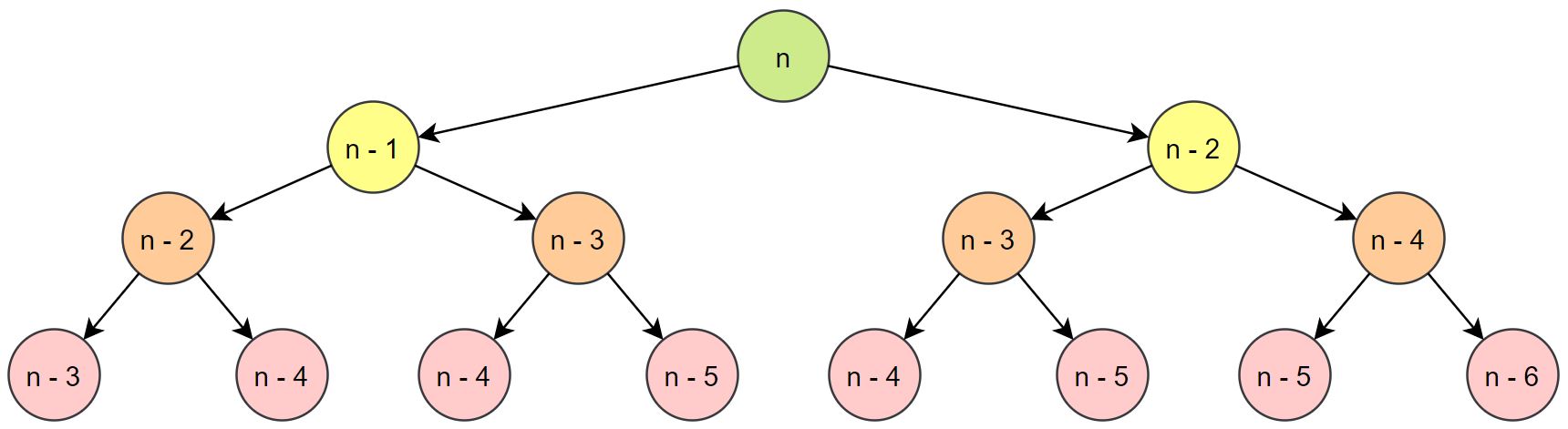
Clearly recursiveFib is repeating calculations. Four times it calls itself with input n - 4, when really this should only be calculated once. Observe adjacent layers a and b of the tree, where a is immediately above b, with x and y nodes respectively. Then we see that y = 2x. As n increases in size, the number of calls recursiveFib makes to itself grows significantly. Surely there’s a better approach for solving this problem?
Consider the initial Fibonacci numbers fib(0) = 0 and fib(1) = 1. Adding them together gives us fib(2) = 1. With fib(1) and fib(2) now known to us, we may add them to obtain fib(3) = 2. Following this pattern, remembering only the last two Fibonacci numbers found, we eventually reach fib(n). This is the DP approach.
public static long dpFib(int n) {
  long prevFibNum = 0;
  long currFibNum = 1;
  long tempVar;
  int index = 1;

  if (n == 0) return prevFibNum;

  while (index < n) {
    tempVar = currFibNum;
    currFibNum += prevFibNum;
    prevFibNum = tempVar;
    index++;
  }

  return currFibNum;
}
Starting with the first two numbers in the sequence, the DP algorithm computes each Fibonacci number exactly once, and only ever remembers the last two found. At no point do we repeat calculations to obtain fib(n), making this much more efficient than the recursive algorithm before. With this elementary example in mind, let’s move away from individual numbers and instead consider work on matrices.
Traversing a Matrix
Suppose we’re driving a bus, and we’re given a 4 x 5 matrix corresponding to areas (or cells) enclosed by grid lines on our map. Each cell covers one bus stop, and each one holds a non-negative number to show how many passengers are waiting to board the bus at this stop.
| 3 | 5 | 0 | 3 | 1 |
|---|---|---|---|---|
| 4 | 2 | 0 | 2 | 4 |
| 5 | 0 | 4 | 0 | 2 |
| 2 | 1 | 1 | 0 | 0 |
Starting from the top-left corner of the map, the final destination for this bus is on the bottom-right corner. In order for the bus to reach its destination on time, the bus may drive only to the right or downward. Assuming the bus can pick up everyone it reaches, we wish to determine the maximum number of people this bus can pick up before arriving at its final destination.
Let’s consider the start of the journey at the top-left corner. The bus starts there, so it must pick up those three passengers. With them on board, we now have a choice on our hands - to travel right or to travel down. One (if not both) of these directions will help us to obtain the maximum possible number of passengers. For the bus to pick up as many people as possible, we need to work out which path to follow in order to achieve this. Every possible journey must be considered. Can we do this scanning the matrix only once? Of course!
Assuming the map to hold at least one cell, we introduce a new matrix maxPassengers holding the same dimensions as the map. Since we must pick up everyone at our starting location, the top-left cell of maxPassengers will be equal to the top-left cell of the map. Given the initial number of passengers, and the fact that the bus may only travel right or down, we know that for each cell in the top row of the map, the bus must arrive from the left. Therefore the maximum number of passengers at each of those cells must be the sum of passengers from the starting position to that cell.
maxPassengers[0][0] = map[0][0];

for (int c = 1; c < numColumns; c++) {
  maxPassengers[0][c] = map[0][c] + maxPassengers[0][c - 1];
}
A similar logic is applied to the first column of cells in the map, where the bus may only arrive from above.
for (int r = 1; r < numRows; r++) {
  maxPassengers[r][0] = map[r][0] + maxPassengers[r - 1][0];
}
Starting from cell (1, 1), and traversing from left to right, row-by-row, the algorithm can populate the remaining rows and columns to work out the maximum possible number of passengers at any point. For each remaining cell, the algorithm knows the bus can only arrive from above, or from the left. Therefore the maximum number of passengers for each cell is the maximum from the left or above, plus the number of passengers waiting at that cell.
for (int r = 1; r < numRows; r++) {
  for (int c = 1; c < numColumns; c++) {
    maxPassengers[r][c] = map[r][c] + Math.max(maxPassengers[r - 1][c], maxPassengers[r][c - 1]);
  }
}
With each of these code segments combined, we have our complete DP algorithm to traverse the map exactly once. When the cell at the bottom-right corner (i.e. our final destination) is populated, we have our answer.
public static int maxPassengerPickup(int[][] map) {
  int numRows = map.length;

  if (numRows == 0) return 0;

  int numColumns = map[0].length;

  int[][] maxPassengers = new int[numRows][numColumns];

  maxPassengers[0][0] = map[0][0];

  for (int c = 1; c < numColumns; c++) {
    maxPassengers[0][c] = map[0][c] + maxPassengers[0][c - 1];
  }

  for (int r = 1; r < numRows; r++) {
    maxPassengers[r][0] = map[r][0] + maxPassengers[r - 1][0];
  }

  for (int r = 1; r < numRows; r++) {
    for (int c = 1; c < numColumns; c++) {
      maxPassengers[r][c] = map[r][c] + Math.max(maxPassengers[r - 1][c], maxPassengers[r][c - 1]);
    }
  }

  return maxPassengers[numRows - 1][numColumns - 1];
}
In the end, our bus was able to pick up a grand total of 19 people. We’re unlikely to outperform Megabus or Citylink any time soon, but it definitely could be worse! Here’s the route followed by the algorithm to reach that result:
| 3 | 5 | 0 | 3 | |
|---|---|---|---|---|
| 2 | 4 | |||
| 2 | ||||
| 0 |
Matrix Chain Multiplication
With numbers and individual matrices covered, let’s move on to consider an entire chain of matrices! This example is a particularly complicated one, so bear with me whilst I try to dive into the details. At the very least, I wish to convey the general purpose of DP for this problem, even if I obfuscate the details of the algorithm.
Consider the following scenario: We have four matrices, named A, B, C, and D, with dimensions 30 x 14, 14 x 15, 15 x 20, and 20 x 10 respectively. We wish to compute the matrix chain ABCD. One possible approach to obtaining ABCD would be to calculate AB, followed by ABC, followed by ABCD. In order words, computing ((AB)C)D.
Given any pair of matrices X and Y with dimensions m x n and n x q respectively, multiplying them to obtain chain XY requires m x n x q arithmetic operations, leaving us with a m x p matrix. Therefore calculating ((AB)C)D requires
    cost(AB) + cost((AB)C) + cost(((AB)C)D)
  = 30 * 14 * 15 + 30 * 15 * 20 + 30 * 20 * 10
  = 6300 + 9000 + 6000
  = 21300
arithmetic operations. However, matrix multiplication is associative, meaning that (XY)Z = X(YZ), so there’s more than one approach to solving this problem. Is our approach from left to right the most efficient one we can take? We have a total of five options to consider:
| Approach | Equation | # Operations |
|---|---|---|
| ((AB)C)D | 30 * 14 * 15 + 30 * 15 * 20 + 30 * 20 * 10 | 21300 |
| A(B(CD)) | 15 * 20 * 10 + 14 * 15 * 10 + 30 * 14 * 10 | 9300 |
| (AB)(CD) | 30 * 14 * 15 + 15 * 20 * 10 + 30 * 15 * 10 | 13800 |
| A((BC)D) | 14 * 15 * 20 + 14 * 20 * 10 + 30 * 14 * 10 | 11200 |
| (A(BC))D | 14 * 15 * 20 + 30 * 14 * 20 + 30 * 20 * 10 | 18600 |
It turns out our original approach required the most arithmetic operations! The most efficient approach would be to compute A(B(CD)), which involves 9300 arithmetic operations. This pattern doesn’t necessary hold for all cases - the answer is dependent entirely on the dimensions of the matrices provided. As the number of matrices involved grows, so do the number of possible approaches to performing the multiplication. So how could we work out the most efficient approach for any chain of matrices? You guessed it - DP!
The DP approach to this problem considers first the base case: If we only have two matrices to multiply, then multiply them. Otherwise, from left-to-right, determine the cost of multiplying every pair of adjacent matrices in the sequence. Following our example, this would be AB, BC, and CD.
Having worked out the minimal costs for each pair, the DP algorithm moves on to consider all possible chains of length three: ABC, and BCD. For each of these chains, there’s two points where we could split them into two separate matrices: ABC has A(BC) and (AB)C, whilst BCD has B(CD) and (BC)D. There’s no need to break this down any further since we already know the minimal costs of computing each parenthesised pair!
Assume the algorithm has determined the most efficient approach to computing ABC and BCD. The next steps will explain the same approach used, but in greater detail. The algorithm proceeds to determine the minimal cost of computing each possible chain of length four. In this example, we have only one: ABCD. There’s three positions where we can split ABCD down into two smaller matrix chains: A(BCD), (AB)(CD), and (ABC)D. The algorithm already knows the minimal cost for computing each parenthesised chain, as before.
Given this chain of length n to begin with, the DP algorithm defines a table M of size n x n to hold the minimal costs it computes. Indexing each position in the chain from 0 -> n - 1, cell (i, j) holds the minimal cost for the matrix chain which starts at position i and terminates at position j (inclusive). Keeping this in mind, M in our example at this stage would appear as follows:
| A: 0 | AB: 6300 | ABC: 12600 | ABCD: ? |
|---|---|---|---|
| B: 0 | BC: 4200 | BCD: 5100 | |
| C: 0 | CD: 3000 | ||
| D: 0 |
Once determined, the minimal cost for computing ABCD will be held in the upper-right corner. So what’s the procedure to follow in order to determine this cost? Remember, the only chains we care about at this stage are A and BCD from A(BCD), AB and CD from (AB)(CD), and ABC and D from (ABC)D. Let’s discard the minimal costs for other chains, and revisit our table:
| A: 0 | AB: 6300 | ABC: 12600 | ABCD: ? |
|---|---|---|---|
| BCD: 5100 | |||
| CD: 3000 | |||
| D: 0 |
The costs to consider for computing ABCD may be broken down as follows:
- A(BCD): cost of A + cost of BCD + cost of computing A(BCD)
- (AB)(CD): cost of AB + cost of CD + cost of computing (AB)(CD)
- (ABC)D: cost of ABC + cost of D + cost of computing (ABC)D
Using index p to iterate over each approach (i.e. p: 0 -> 2), the algorithm considers matrix chains X (from position 0 to p) and Y (from p + 1 to 3) from M. The minimal costs corresponding to X and Y in M are held in cells (0, p) and (p + 1, 3) respectively. Highlighting the pair fetched for approach (1) in blue, (2) in red, and (3) in green, we observe a pattern in how previous calculations are fetched:
| A: 0 | AB: 6300 | ABC: 12600 | ABCD: ? |
|---|---|---|---|
| BCD: 5100 | |||
| CD: 3000 | |||
| D: 0 |
Given the minimal costs of both matrix chains to be multiplied together, the algorithm is left to work out the cost of performing the multiplication itself. Remember, if X and Y have dimensions m x n and n x q respectively, multiplying them to together to obtain chain XY requires m x n x q arithmetic operations. Therefore we require the number of rows m in X, the number of columns (equivalent to the number of rows) n in Y, and the number of columns q in Y.
Suppose we’re given the dimensions of our matrices as an array called dims of length n + 1, where element 0 <= i < n holds the number of rows in the (i + 1)th matrix, and element n holds the number of columns in the nth matrix of the chain. Following our example ABCD, dims would be [30, 14, 15, 20, 10].
For each possible splitting of chain ABCD, again using p: 0 -> 2, we require the number of rows in the first matrix A, the number of columns in the matrix at position p (equivalent to the number of rows in matrix p + 1), and the number of columns in the last matrix D. In other words, we require dims(0), dims(p + 1), and dims(4). The cost for each approach to computing ABCD may now be defined as follows:
- A(BCD): cell(0, 0) + cell(1, 3) + dims(0) * dims(1) * dims(4)
- (AB)(CD): cell(0, 1) + cell(2, 3) + dims(0) * dims(2) * dims(4)
- (ABC)D: cell(0, 2) + cell(3, 3) + dims(0) * dims(3) * dims(4)
Substituting in the numbers from M and dims, we have:
- A(BCD): 0 + 5100 + 30 * 14 * 10 = 0 + 5100 + 4200 = 9300
- (AB)(CD): 6300 + 3000 + 30 * 15 * 10 = 6300 + 3000 + 4500 = 13800
- (ABC)D: 12600 + 0 + 30 * 20 * 10 = 12600 + 0 + 6000 = 18600
There we have it - confirmation that the answer is 9300! In addition to table M, the algorithm populates a second table, S, which is the same size as M. For each matrix chain considered by the algorithm, the position in which it is split into two smaller chains is stored in S in a cell sharing the same row and column indices as the cell in M holding the chain’s minimal cost. Along with these two tables, the algorithm uses four additional variables worth noting:
chainLeniterates over the range of chain lengths to consider, from 2 to niiterates over each chain X of lengthchainLencontained in the given chaincolumnindicates the column index for X in tables M and Sp, as before, iterates over each position where X is split into two smaller chains
With these variables defined, the full implementation of matrix chain multiplication is as follows:
public static void matrixChainMulOrder(int[] dims) {
  int n = dims.length - 1;
  int[][] M = new int[n][n];
  int[][] S = new int[n][n];
  int cost;
  int column;

  for (int chainLen = 2; chainLen <= n; chainLen++) {
    for (int i = 0; i < n - (chainLen - 1); i++) {
      column = i + chainLen - 1;
      M[i][column] = Integer.MAX_VALUE;

      for (int p = i; p < column; p++) {
        cost = M[i][p] + M[p + 1][column] + dims[i] * dims[p + 1] * dims[column + 1];

        if (cost < M[i][column]) {
          M[i][column] = cost;
          S[i][column] = p;
        }
      }
    }
  }
}
Not the most straightforward application, but nevertheless pretty cool, right?
Conclusion
DP holds an abundance of applications. This post only scrapes the surface with the three examples provided. Whilst these algorithms I think suffice for demonstrating the elegance of DP, another application of particular interest to me is the Viterbi algorithm for anyone wishing to read into DP further. If you’re keen to practice DP, Codility offers two good and challenging exercises in lesson 17, whilst more opportunities of varying difficulty may be found by signing up to Code Wars.
