
Introduction
The task today is to process the London Cycle Hire data into two separate sets, Weekends and Weekdays. Grouping data into smaller subsets for further processing is a common business requirement and we’re going to see how Spark can help us with the task.
The data consists of 167 CSV files, totalling 6.5GB, and we will be processing it using a two node cluster, each with 4GB of RAM and 3 CPUs.
Before we begin processing the real data, it is useful to understand how Spark is moving our data around the cluster and how this relates to performance. Spark is unable to hold the entire dataset in-memory at once and therefore must write data to a drive or pass it across the network. This is much slower than in-memory processing and it is here where bottlenecks commonly occur.
In Theory
Partitioning
To distribute work across the cluster and reduce the memory requirements of each node, Spark will split the data into smaller parts called Partitions. Each of these is then sent to an Executor to be processed. Only one partition is computed per executor thread at a time, therefore the size and quantity of partitions passed to an executor is directly proportional to the time it takes to complete.
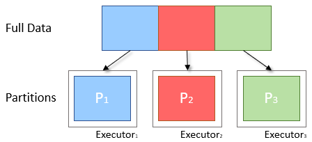
Fig: Diagram of Ideal Partitioning
Data Skew
Often the data is split into partitions based on a key, for instance the first letter of a name. If values are not evenly distributed throughout this key then more data will be placed in one partition than another. An example would be:
{Adam, Alex, Anja, Beth, Claire}
-> A: {Adam, Alex, Anja}
-> B: {Beth}
-> C: {Clair}
Here the A partition is 3 times larger than the other two, and therefore will take approximately 3 times as long to compute. As the next stage of processing cannot begin until all three partitions are evaluated, the overall results from the stage will be delayed.
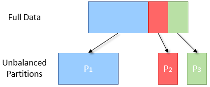
Fig: Diagram of Skewed Partitioning
Scheduling
The other problem that may occur when splitting into partitions is that there are too few partitions to correctly cover the number of executors available. An example is given in the diagram below, in which there are 2 Executors and 3 partitions. Executor 1 has an extra partition to compute and therefore takes twice as long as Executor 2. This results in Executor 2 being idle and unused for half the job time.
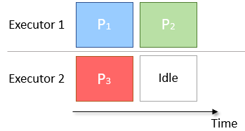
Fig: Diagram of Badly Scheduled Partitioning
Solution
The simplest solution to the above two problems is to increase the number of partitions used for computations. This will reduce the effect of skew into a single partition and will also allow better matching of scheduling to CPUs.
A common recommendation is to have 4 partitions per CPU, however settings related to Spark performance are very case dependent, and so this value should be fine-tuned with your given scenario.
Shuffling
A shuffle occurs when data is rearranged between partitions. This is required when a transformation requires information from other partitions, such as summing all the values in a column. Spark will gather the required data from each partition and combine it into a new partition, likely on a different executor.
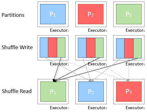
Fig: Diagram of Shuffling Between Executors
During a shuffle, data is written to disk and transferred across the network, halting Spark’s ability to do processing in-memory and causing a performance bottleneck. Consequently we want to try to reduce the number of shuffles being done or reduce the amount of data being shuffled.
Map-Side Reduction
When aggregating data during a shuffle, rather than pass all the data, it is preferred to combine the values in the current partition and pass only the result in the shuffle. This process is known as Map-Side Reduction and improves performance by reducing the quantity of data being transferred during a shuffle.
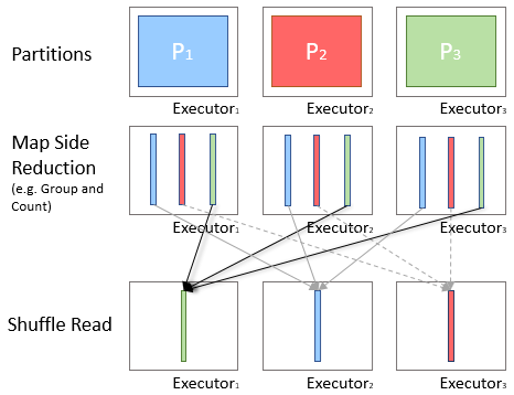
Fig: Diagram of Map-Side Reduction
Spark developers have put a lot of work into improving the automatic optimisation offered by Spark, in particular the Dataset groupBy function will perform map-side reduction automatically where possible. However it is still necessary to check the execution diagrams and statistics for large shuffles where reduction did not occur.
In Practice
To split the data, we are going to add a column that converts the Start Date to a day of the week, Weekday, and then add a boolean column for whether the day is a weekend or not, isWeekend. The data also requires some cleaning to remove erroneous Start Dates and Durations.
Dataset<Row> data = getCleanedDataset(spark);
data = data.withColumn("Weekday",
              date_format(data.col("Start_Date"), "EEEE"));
data = data.withColumn("isWeekend",
       data.col("Weekday").equalTo("Saturday")
              .or(data.col("Weekday").equalTo("Sunday")));
Finally, we will repartition the data based on the isWeekend column and then save that in Parquet format.
data.repartition(data.col("isWeekend")).write()
        .parquet("cycle-data-results" + Time.now());
Round 1
When the job is run, we see the repartition command does a shuffle and produces 200 partitions (the spark default), which should offer excellent levels of parallelisation; let’s look at the execution timeline.
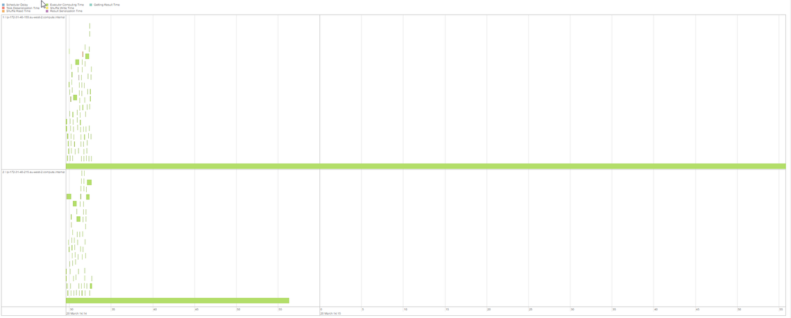
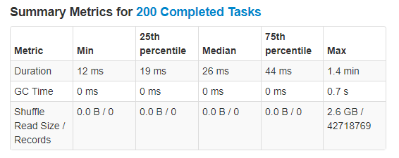
Fig: 200 Partitions Execution Timeline and Metrics
The timeline does not look balanced. There are only two partitions taking up any significant execution time, amongst many very tiny ones, and even between the two larger ones the processing is not equally split, if anything they look like they have a ratio of roughly 5 to 2. This is indicative of data skew, as the partitions are taking different lengths of time to process, and also demonstrates the scheduling issues mentioned before, with the second executor being idle for the last 60 seconds.
This unequal split of processing is a common sight in Spark jobs, and the key to improving performance is to find these problems, understand why they have occurred and to rebalance them correctly across the cluster.
Why?
In this case it has occurred because calling repartition moves all values for the same key into the same partition on one Executor. Here our key isWeekend is a boolean value, meaning that only two partitions will be populated with data. Spark is not able to account for this in its internal optimisation and therefore offers 198 other partitions with no data in them. If we had more than two executors available, they would receive only empty partitions and would be idle throughout this process, greatly reducing the total throughput of the cluster.
Grouping in this fashion is also a common source of memory exceptions as, with a large data set, a single partition can easily be given multiple GBs of data and quickly exceed the allocated RAM. Therefore we must consider the likely proportion of data for each key we have chosen and how that correlates to our cluster.
Round 2
To improve on the above issues, we need to make changes to our query so that it more evenly spreads the data across our partitions and executors.
Another way of writing the query is to delegate the repartitioning to the write method.
data.write().partitionBy("isWeekend")
        .parquet("cycle-data-results" + Time.now());
In the previous case Spark loaded the CSV files into 69 partitions, split these based on isWeekend and shuffled the results into 200 new partitions for writing. In the new solution Spark still loads the CSVs into 69 partitions, however it is then able to skip the shuffle stage, realising that it can split the existing partitions based on the key and then write that data directly to parquet files. Looking at the execution timeline, we can see a much healthier spread between the partitions and the nodes, and no shuffle occurring.
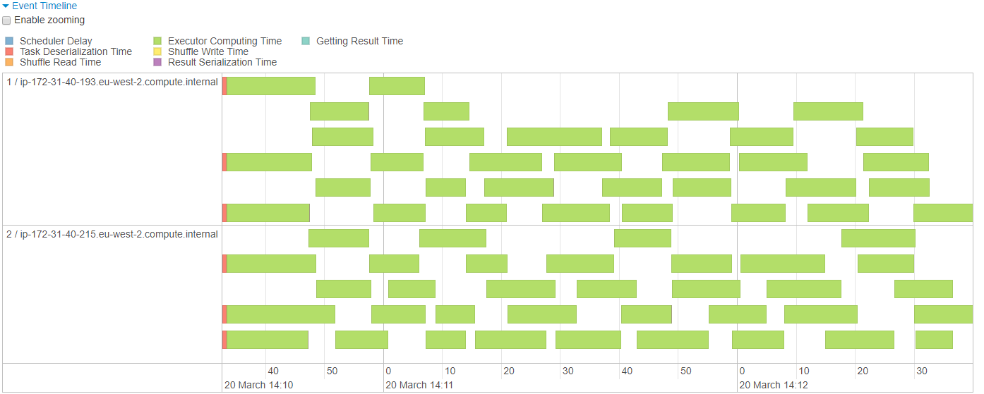
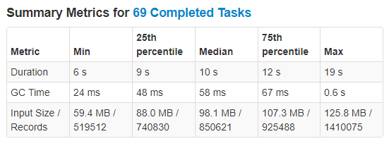
Fig: Improved Execution Timeline and Metrics
Conclusion
In this case the writing time has decreased from 1.4 to 0.3 minutes, a huge 79% reduction, and if we had a cluster with more nodes this difference would become even more pronounced. Further to that we have avoided 3.4GB of Shuffle read and write, greatly reducing the network and disk usage on the cluster.
Hopefully this post has given some insight into optimising Spark jobs and shown what to look for to get the most out of your cluster.
A repository with the example code can be found here.

