If you’re a connoisseur of science fiction, you may believe that “quantum” is just a magic word. An enchanted word that makes computers omnipotent, allows you to break the barriers of time and turn Internet Explorer into a decent browser. These are all of-course equally improbable. However, the physics of quantum mechanics does have many uses. One such application is quantum computing. In this post, I discuss what quantum computing is, why nations and corporations are investing millions, and the significant hurdles currently stopping us from realising the full potential.
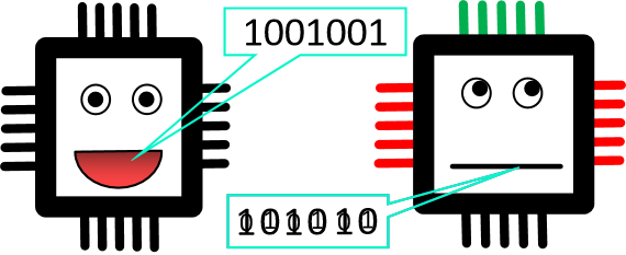 The new quantum kids with their strange way of talking show great potential. However, they aren’t yet well behaved enough to actually get a job.
Dehype the hype!
Let’s first challenge some misconceptions. Quantum computing will not just make everything go faster. So if you are here because you want your Windows updates to run faster, I’m sorry. For most everyday things, quantum computers would probably run slower than classical (or “normal”) ones. Quantum computers also can’t do any computation that a classical computer can’t. We know this because we can simulate quantum computers on classical ones, albeit very slowly. There is a lot of misleading claims online that talk about problems that classical systems “can’t solve” when they mean “can’t solve efficiently”.
The truth about quantum computers is they are a breed of computers fundamentally different from classical ones. This difference means they run a class of programs dissimilar to those run on classical computers. Even though the programs are distinct, they can often be used to solve the same problems. For some of these problems, the quantum computer/programs outperform their classical analogue. The difference isn’t just about getting the answers slightly faster. They could perform calculations on a useful timescale that would otherwise take millions of years.
How does a quantum computer beat classical computers?
Classical Computers
At the smallest level of logic, classical computers deal with bits and logic gates. Everything your computer does, stores and shows is nothing more than bits and logic gates.
A bit is the smallest unit of information. It has two possible states, often referred to as “0 and 1”, or “on and off”. Physically a bit can be stored in any device that can be in one of two possible states. Examples include two distinct voltage levels allowed by a circuit, two directions of magnetisations, and different levels of light intensity.
Logic gates perform operations on these bits. Each logic gate is like a function that takes in one or two bits and outputs one bit. For example, the AND gate takes in two bits and outputs a 1 if and only if both inputs are a 1, else it outputs a 0.
Quantum Physics
Recently (by which I mean since the start of the 20th century), physicists have been studying the strange behaviour of tiny things. Here are a couple of relatively simple (simple to understand the effects of, not the causes) examples. The single particle double slit experiment demonstrates that a quantum particle, like an electron, fired at a sheet with 2 slits close together, will go through both slits simultaneously. It will be in 2 places at the same time. In quantum tunnelling a particle may go from one state to another, even if it does not have the energy. This is like if a ball spontaneously went through a hill to get to the valley on the other side because it didn’t have the energy to jump over. A quantum computer exploits this strange world to gain its advantage.
If anything you read about this feels absurd, that is good! It is counter-intuitive because our experiences are all to do with the world at “normal” scales.
Superposition
Superposition is a fundamental principle of quantum physics that quantum computers exploit. A qubit (quantum bit) can, like a bit, be 0 or 1. But it can also be in a superposition of 0 and 1. A superposition means the qubit is both a 0 and a 1.
It is practical to use the proper notation (known as bra-ket notation).
-
A qubit in the 0 state is represented by \(\ket{0}\).
-
A qubit in the 1 state is represented by \(\Ket{1}\).
-
A superposition is represented by \(a_0\Ket{0} + a_1\Ket{1}\).
-
The values \(a_0\) and \(a_1\) are (complex) coefficients.
-
\(\Ket{x}\) is known as a ket.
You can measure a qubit to check its state. If the qubit is in a superposition, the measurement causes the qubit to collapse. This means the qubit randomly “chooses” to become a 1 or a 0. In essence, it tricks the measuring device. The coefficients in \(a_0\Ket{0} + a_1\Ket{1}\) determine how likely it is for the qubit to choose 0 or 1 1. After the measurement, the qubit will remain in the new state. In general, there is no way to determine \(a_0\) and \(a_1\) or which way the qubit will collapse.
This may make it seem like superposition isn’t real, and that the qubit was always in the state we found after measurement. However, the uncertainty is actually in the fabric of the universe. You can try to convince yourself of this by reading about the double-slit experiment linked above.
Now let’s say we have two qubits, the first is the state \(a_0\Ket{0} + a_1\Ket{1}\) and the second is in the state \(b_0\Ket{0} + b_1\Ket{1}\). We can combine them by multiplying them together (formally known as taking the tensor product)
\[(a_0\Ket{0} + a_1\Ket{1})(b_0\Ket{0} + b_1\Ket{1}) =\] \[a_{0}b_{0}\ket{0}\ket{0} + a_{0}b_{1}\ket{0}\ket{1} + a_{1}b_{0}\ket{1}\ket{0} + a_{1}b_{1}\ket{1}\ket{1} =\] \[a_{0}b_{0}\ket{00} + a_{0}b_{1}\ket{01} + a_{1}b_{0}\ket{10} + a_{1}b_{1}\ket{11} =\] \[a_{0}b_{0}\ket{0} + a_{0}b_{1}\ket{1} + a_{1}b_{0}\ket{2} + a_{1}b_{1}\ket{3}\]Note that \(\ket{0}\ket{1}\) and \(\ket{1}\ket{0}\) are two different terms. The last two lines demonstrate the flexibility in the notation. We can reduce \(\ket{0}\ket{0}\) into a single ket. And the contents of the ket only have to tell us the overall state. In this example, I converted the binary numbers to their decimal notation. I could also just rename \(00\) to \(blue\) etc.
Sidenote: Superposition is often represented via a Bloch sphere. It can help create a visual analogy for superposition in a single qubit, but I avoid it because it can be misleading and it isn’t as helpful when it comes to entanglement.
Entanglement
You might have heard about entanglement. It is usually explained through Einstein’s thought experiment ‘spooky action at a distance’. Imagine we have the 2-qubit entangled state,
\[\ket{00} + \ket{11}\]If we were to measure the first qubit, we have a 50/50 chance of getting a 0 or 1. The measurement causes the state to collapse instantly. This means that the state of the second qubit immediately changes to match the first. Even if we took the two qubits and put them on different planets, measuring one would instantly affect the other. So we have faster than light communication? Not really! There is no way to force the measurement to go a certain way. And no way to know whether the qubit has already collapsed. So there isn’t a way we can use this to communicate. We know that the state isn’t determined in advance, as demonstrated by something called Bell inequalities 2.
When qubits become entangled, it no longer makes sense to consider each qubit individually. To understand what this means, recall the equation,
\[(a_0\Ket{0} + a_1\Ket{1})(b_0\Ket{0} + b_1\Ket{1}) =\] \[a_{0}b_{0}\ket{00} + a_{0}b_{1}\ket{01} + a_{1}b_{0}\ket{10} + a_{1}b_{1}\ket{11} =\]and consider what values of \(a_0\), \(a_1\), \(b_0\) and \(b_1\) give us our entangled state (\(a_{0}b_{1} = a_{1}b_{0} = 0\) and \(a_{0}b_{0} = a_{1}b_{1} = 1\)). There is no solution. So it no longer makes sense to ask what the state of an individual qubit is3. Entanglement is important because it opens up the list of allowed states to any superposition of inputs. The information represented in the state increases exponentially4
Linear Operators
A crucial part of quantum computing is that operations are linear. To understand what this means, imagine you have a quantum machine set up to calculate square numbers. So if you set the qubits to represent \(\ket{2}\), when the machine finishes the qubits will say \(\ket{4}\). This calculation can be done without any measurement. This fact along with the operators being linear means that if the initial state is
\[a_0\ket{0} + a_2\ket{2} + a_5\ket{5}\]the output will be
\[a_0\ket{0} + a_2\ket{4} + a_5\ket{25}\]This is key! An operation on a superposition of inputs results in an alike superposition of their individual outputs. This gives us parallel computing. Importantly the parallel computing is free. By this I mean, if you make a quantum system for a function it can automatically support parallel computing on all possible inputs. At this point, you may recall that if we had qubits in this state, we would not be able to determine the full state (unless we used a slow classical simulation). We would only be able to measure it and get one of the values in the superposition randomly. So how can we make any use of this parallel computing? Some insight is given in the next section.
The types of quantum computing
There are a lot of ways to do quantum computing and a lot of ways to categorise those ways. There is also some overlap and confusion about definitions. Still, I have selected a few “types” of quantum computing to explain.
Quantum Simulations
As discussed above, the intrinsic nature of the very small is counter-intuitive and bizarre. Running simulations would be an excellent way of gaining more insights. However given the enormous amounts of information that exists in quantum systems, simulating things on a classical computer is very slow. Quantum computer would be superior at running simulations of things like molecules. They could unlock secrets that would have a huge impact on the world. Examples include making fertilisers more efficiently (currently its production causes 3% of global CO2 emissions), finding materials to create more efficient solar panels and creating better carbon capture. Learn more here and here.
Quantum Annealing
Quantum annealing solves optimisation problems by using the fact that the universe is perpetually solving optimisation problems. An optimisation problem is one where you are trying to find the best solution from all potential solutions. For example, finding the quickest route for a journey. In this case, we refer to the duration as the “objective variable”. Our goal is to minimise the objective variable, while not violating the constraints. Constraints are restrictions that the final solution must fulfil. For example staying on roads, avoiding tolls, and not messing with the fabric of reality (using a flux capacitor, 1.21 gigawatts of power and 88mph of speed).
We can rewrite an optimisation problem as an energy minimisation problem. We apply a field to the qubits (e.g. a magnetic field) in such a way that different states have different energies. We set it up so that better solutions have lower energies. It may sound like this means we already know the solution, however simply knowing the problem statement gives you enough information to set up the field. The lowest energy state of a particular configuration is known as the ground state. Each configuration has a different ground state and it always corresponds to the best possible solution.
To solve a problem we set up the field such that the ground state is an equal superposition of all configurations and make sure the system is in the said ground state. Then slowly evolve the field to match the one that describes our problem. In an ideal setup, the qubits will always be in the ground state of the current setup and therefore represent the correct solution when measured at the end. In reality, there is a non-zero chance that the qubits will jump to a higher energy state, however, there is still hope that this method can give us a “good enough” solutions faster than classical means.
To understand this better, consider the diagram of a super-simplified one qubit example. At first, the ground state is an equal superposition. Then we evolve the system so that the 1 state becomes the ground state. When this qubit is measured, it is more likely to be a 1, because the system tends to stay in the lowest energy state.
![Quantum annealing energy diagram]](/garora/assets/2020-09-23/annealing.png)
Quantum annealing has potential applications in predicting financial markets, detecting fraud, machine learning and a whole lot more.
Universal Quantum Computing (Circuit Model)
A universal quantum computer would be able to solve any problem that any quantum paradigm can solve. It is the hardest to make. The circuit model is the most popular way of realising universal quantum computing. It is also relatively simple to grasp because of its similarity to classical computers. Analogous to classical computing, quantum gates are the foundations of all possible computations. One key difference between classic and quantum gates is that quantum gates never output a new qubit based on the input, but manipulate the qubits already there.
Experts are always looking for new quantum solutions to problems. So it’s difficult to be precise about what kind of problems quantum computers will be able to solve efficiently. But I can try to give a feeling for it. Useful quantum algorithms will make use of parallel computing. However, if you need to know the result of each calculation, quantum computing won’t help. The quantum advantage comes when you want to combine the results to get the final answer. Here are two examples:
Grover’s Algorithm
Grover’s algorithm is for inverting a function. Sometimes there isn’t an efficient way to classically invert a function. Let’s explain this with square numbers (this is just an example, inverting the square is very easy). Imagine you wanted to know the square root of 529, and the only way was to try squaring all the numbers from 0 to 30 and checking each one, one after the other. Grover’s algorithm offers a quicker solution.
To use Grover’s algorithm we need a quantum circuit called a Grover oracle. The Grover oracle is encoded with the function that we aim to invert (squaring) and the target value (529). The job of the Grover oracle is to take an input and ‘mark’ it if it satisfies our condition (squares to give 529). To begin, we give the Grover oracle a balanced superposition of all the potential inputs. It will return the superposition with the correct answer marked (because of linear operators). The next step ‘mixes’ up the probabilities. The ‘mixing’ isn’t uniform, it changes the probability to favour the marked state. A key point is that Grover’s algorithm, like our naive approach, also checks every potential solution. It just does them all in parallel.
The details of ‘marking’ and ‘mixing’ are too advanced for this post, but I encourage you to seek them out for yourself. Grover’s algorithm isn’t guaranteed to give the correct answer, but, because the answers are easy to check, you can expect the correct solution after a few tries. Even with having to do repeats, it is quicker.
Shor’s Algorithm
Shor’s algorithm is for finding the factors of numbers efficiently. This could break some of the most widely used encryption algorithms. I won’t go into all the details, but instead, discuss an analogy to illustrate a crucial part. Let’s imagine you have an enormous list of people. They all have hats. The colours of the hats repeat regularly e.g. red, blue, black, red, blue, black….. The periodicity of this is three because every three people the pattern resets. Now imagine a function that given a number tells you the colour of the person in that position. How do you find the period? Classically you would cycle through numbers until you find where repetition happens.
To use quantum computing, we need some qubits to encode a number and a colour. And the function needs to be able to convert \(\ket{x, blank}\) to \(\ket{x, colour\:at\:x}\). The first step is to start in a full superposition of all inputs with no colour,
\[\ket{1, blank} + \ket{2, blank} ... + \ket{N, blank}\]where N is the number of people in the line. This state, after applying the function, will become (for example)
\[\ket{1, red} + \ket{2, green} ... + \ket{N, white}\]Next, we need to make a careful measurement. Measurements do not have to measure everything. We can measure the qubits that represent the colour on their own. The result is that the colour is randomly selected, and all states that are not related to that colour vanish. For example, we could get,
\[\ket{288, black} + \ket{588, black} ... + \ket{3588, black}\]The colour doesn’t matter here. The key is that all the numbers have constant spacing (the period). If we were to measure the number, it would just give a random number, which is of no use. However, a quantum Fourier transform can be used to determine the periodicity.
How to use a quantum computer
We’ve discussed qubits in theory, let’s look at the practical. There are many ways to implement a quantum computer. One way is a trapped ion quantum computer. In this, ions (charged atomic particles) are the qubits, and lasers perform operations. This means all calculations are a series of laser instructions and measurements. Other examples include using current carrying loops as qubits which are controlled by a magnetic field, and dissolved molecules as qubits manipulated with radiowaves. So when you program a quantum computer you are programming the part of the machine that controls the lasers/radio waves/magnetic fields. How do you do this?
Your quantum computer won’t come with a screen, and you can’t just connect your keyboard and start typing in code. Instead, you would use a regular computer with access to the quantum device. This is similar to how you might get a shared supercomputer to run some code. It is common to write code on your regular computer, test the code on a smaller problem and then send the code to the supercomputer to run. Similarly, you could test your quantum code on a small calculation using a classical simulation and then pass it to the quantum computer. A key difference is a supercomputer tends to have a common piece of software to your device, which it uses to run the code. But for a quantum computer, you have to translate the code into instructions for whatever is controlling the qubits (e.g.lasers).
Just some of the challenges
The most significant hurdle to unleashing the potential of quantum computing is decoherence. Decoherence collapses the quantum state just like a measurement. Depending on the type of qubits, decoherence can be caused by heat, vibrations, light and practically any interaction with the outside world. Even the tools used to perform controlled actions on the qubits aren’t completely reliable. As a result, a lot of time, money, and effort is devoted to the research and implementation of keeping qubits in extreme environments. For example, some qubits need to be at 20 millikelvins (0.002 Celcius above absolute zero).
Manipulating qubits can also require a lot of precision and expertise in the relevant field. As a result, scientists have the task of threading a microscopic needle in gale force winds that keep changing direction while the needle melts.
Another physical restriction is communication between qubits. You might expect that in a quantum computer we can apply a gate on any set of qubits, however, depending on the implementation the possible links can be severely limited. For example, qubits might only be able to interact with their direct neighbours which restricts the complexity of the algorithms that can run on them.
These problems (and more) are currently stopping us from having a quantum computer with enough qubits to be useful from a computational standpoint.
Conclusion
Quantum computers will not solve all your problems. Quantum computers can potentially help change the world. Success is not guaranteed, but that has never been a good enough reason for science to stop.
![Quantum computer developed by IBM Research in Zurich]](/garora/assets/2020-09-23/Zurich_Quantum_Computer.jpg) Quantum computer based on superconducting qubits developed by IBM Research in Zürich, Switzerland. The qubits are cooled to 1 kelvin
Quantum computer based on superconducting qubits developed by IBM Research in Zürich, Switzerland. The qubits are cooled to 1 kelvin
-
In general, these coefficients are complex. The square of the modulus gives the probability that the corresponding state will appear when the qubit is measured. ↩
-
If you watch the video, just imagine a one as spin up and a 0 as spin down. The video explains the conservation of angular momentum forces the spins to be the opposite. To conserve angular momentum in our case, the angular momentum changes inside the measuring devices. ↩
-
Technically, we say that the single qubit is in a “mixed state” however, that is a bit advanced. ↩
-
Once you take into account that coefficients can be complex and that sum of probabilities must be one. Without entangled N qubits can be defined with \(2N\) real numbers and with entanglement you need \(2^{N+1} -1\). ↩