
The purpose of this blog is to look at ways of representing data visually from Elasticsearch. We wish to create reports without exposing the raw data to end users. The aim is to investigate if we can generate visualisations in the cloud in an efficient and cost effective way. We will be using serverless architecture specificially AWS Lambda functions.
Why visualise data?
Visual representations are a clear and concise way of communicating trends and patterns which humans can interpret quickly and easily. Raw numbers can be obscured behind the graph, so they only the trend or generalisation is presented to the user. A bar chart like -
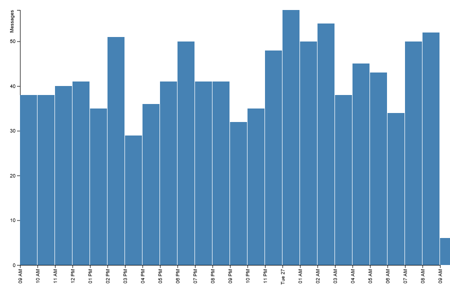 Is a lot easier to analyse than -
    { results: [
        { "key_as_string": "2019-08-26T09:00:00.000Z", "key": 1566810000000, "doc_count": 50 },
        { "key_as_string": "2019-08-26T10:00:00.000Z", "key": 1566813600000, "doc_count": 38 },
        { "key_as_string": "2019-08-26T11:00:00.000Z", "key": 1566817200000, "doc_count": 40 },
        { "key_as_string": "2019-08-26T12:00:00.000Z", "key": 1566820800000, "doc_count": 41 },
        { "key_as_string": "2019-08-26T13:00:00.000Z", "key": 1566824400000, "doc_count": 35 },
        { "key_as_string": "2019-08-26T14:00:00.000Z", "key": 1566828000000, "doc_count": 51 },
        { "key_as_string": "2019-08-26T15:00:00.000Z", "key": 1566831600000, "doc_count": 29 },
        { "key_as_string": "2019-08-26T16:00:00.000Z", "key": 1566835200000, "doc_count": 36 },
        { "key_as_string": "2019-08-26T17:00:00.000Z", "key": 1566838800000, "doc_count": 41 },
        { "key_as_string": "2019-08-26T18:00:00.000Z", "key": 1566842400000, "doc_count": 50 }
    	]
    }
Sample data to visualise
For the purpose of having data to visualaise we have created a mock social media site, which allows for short textual posts with tags. Here is an example of some random machine generated content -
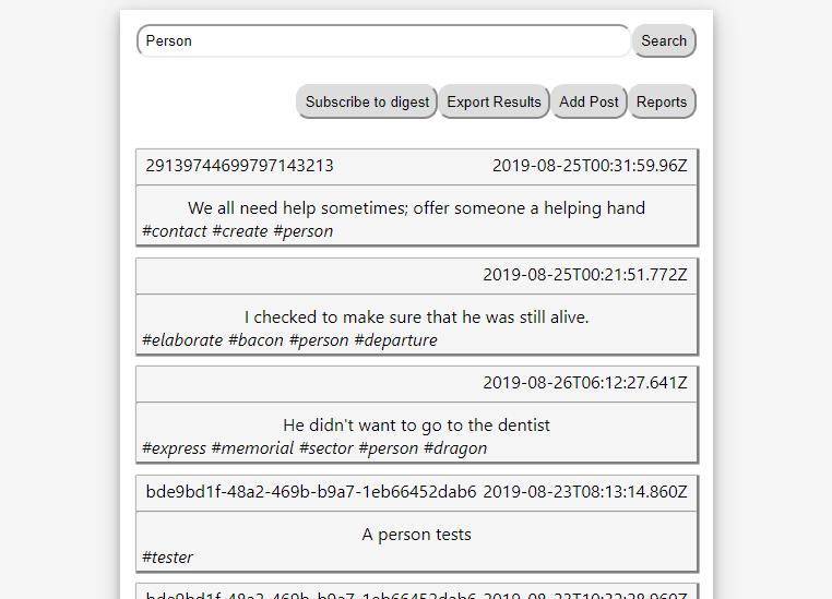
We would like to be able to see and visualise trends which are happening within the system, which can be used to aid marketing or other business decisions.
Selecting the data to show
For this example, we have the potential to have very large data sets. For example Twitter can have approximately 500 million posts a day. We need a method of searching for data which is scalable, so for our example we are using Elasticsearch.
The main advantage to Elasticsearch is you can do sections of aggregation logic within the query itself. For example automatically doing the count per hour of entries, this increases the level of data abstraction, as we dont need to know exactly which entries are included just the aggregate count. Here is an example of the input to reterive the posts per hour for the last 24 hours -
	{
      "aggs": {
        "time_split" : {
            "date_histogram" : {
                "field": "DateCreated",
                "interval": "1h"
            }
        }
      },
      "query" : {
        "bool" : {
            "filter" : [
                { "range" : { "DateCreated": { "gte": "2019-07-21T00:00:00.00Z" } }
                },
                { "range" : { "DateCreated": { "lte": "2019-07-23T00:00:00.00Z" } }
                }
            ]
        }
      }
    }
And here is the response -
	{
      "took": 353,
      "timed_out": false,
      "_shards": { "total": 1,  "successful": 1, "skipped": 0, "failed": 0 },
      "hits": {
        "total": {  "value": 2000, "relation": "eq" },
        "max_score": null,
        "hits": []
      },
      "aggregations": {
        "time_split": {
          "buckets": [
            {
              "key_as_string": "2019-07-21T00:00:00.000Z",
              "key": 1563667200000,
              "doc_count": 27
            }
          ]
        }
      }
  	}
From the Elasticsearch request, there were 2000 matching posts, but the aggreation has split them down to just 24 entries. By moving as much as of the search logic into Elasticsearch we can improve performance, by reducing the total data transfered and the need for manual manipulation of the returned data.
Converting data to visualisations
To make all this data into a user friendly visualisation, we needed to decide what format we wanted the resulting image to be. We believe using an SVG is the correct idea here, as it allows for precise positioning of multiple data points, and it can be scaled in size without becoming distorted like a PNG or JPG would.
We are going to generate an SVG image using a library called D3. We are using SVG as it allow for image scaling without distortion.
Whilst developing we found it easier to develop the D3 code within a web page. D3 has the same API regardless of whether it is used on the client or server. This meant we could develop the code on the client side and be confident it would work when deployed.
The process to produce the SVG follows a typical D3 pattern and can be split down into these sections -

A full example can be found in this file and below is each function in detail.
Prepare Canvas
To prepare the canvas for drawing the D3 visualisation on, we use a fake DOM object. This is the key part which allows us to use D3 within Node.js.
Using the functions provided by D3, we add in the initial SVG element ready to have data drawn onto it -
	_buildContainer() {

        const fakeDom = new JSDOM('<!DOCTYPE html><html><body></body></html>');
        this._body = d3.select(fakeDom.window.document).select('body');
        this._svgContainer = this._body
          .append('div')
          .attr('class', 'container') // class is only needed to grab the element later for returning.
          .append('svg')
          .attr('width', this._width + this._margin.left + this._margin.right)
          .attr('height', this._height + this._margin.top + this._margin.bottom)
          .attr('viewbox', `0 0 ${this._width + this._margin.left + this._margin.right} ${this._height + this._margin.top + this._margin.bottom}`)
          .attr('preserveAspectRatio', 'xMidYMid meet')
          .attr('xmlns', 'http://www.w3.org/2000/svg')
          .append('g')
          .attr('transform', `translate(${this._margin.left}, ${this._margin.top})`);
	}
Create Scales
On the y-scale we will plot a range from 0 to the maximum of the number of posts received, and on the x-scale would be a time scale -
	_buildScales() {

        const dateArray = this._formattedData.map(d => d.formattedDate);
        this._yScale = d3
          .scaleLinear()
          .range([this._height, 0])
          .domain([0, d3.max(this._formattedData, data => data.doc_count)]);
        this._xScale = d3
          .scaleTime()
          .range([0, this._width])
          .domain([dateArray[0], dateArray[dateArray.length - 1]]);
	}
The range variable is the amount of drawable space the image has to plot all the values given. Because of how coordinates work in SVGs, you go from the highest value to lowest on y-scales. yet low to high on x-scales. The domain of the scale is the highest and lowest values which will be plotted against the scale, which can be inferred from the raw data provided.
Draw Axis
Drawing the axis takes the scales from before and convert them to a drawn axis onto the prepared canvas -
	_buildAxis() {
		this._yAxis = d3
          .axisLeft()
          .scale(this._yScale)
          .ticks(5);

      	this._svgContainer
          .append('g')
          .call(this._yAxis)
          .append('text')
          .attr('transform', 'rotate(-90)')
          .attr('y', -6)
          .attr('dy', '-.71em')
          .style('text-anchor', 'end')
          .text('Messages')
          .style('fill', 'black');

        this._xAxis = d3
          .axisBottom()
          .scale(this._xScale)
          .ticks(d3.timeHour);

        this._svgContainer
          .append('g')
          .attr('transform', `translate(0, ${this._height})`)
          .call(this._xAxis)
          .selectAll('text')
          .style('text-anchor', 'end')
          .attr('dx', '-.8em')
          .attr('dy', '-.55em')
          .attr('transform', 'rotate(-90)');
    }
The axis controls how the element should be constructed, and links the scale created above to it, we use this to control what side of the graph the scale will appear, as well as optional elements such as the ‘tick’ marks on the axis. To draw the object to the graph, we append the axis to our prepared canvas, and to help readability we include a label on the axis.
Draw Data
Now we need to pass the data into D3, which we use to draw one rectangle per point -
    _buildContent() {
		this._svgContainer
          .selectAll('bar')
          .data(this._formattedData)
          .enter()
          .append('rect')
          .style('fill', 'steelblue')
          .attr('x', data => this._xScale(new Date(data.formattedDate)))
          .attr('width', this._width / this._formattedData.length)
          .attr('y', data => this._yScale(data.doc_count))
          .attr('height', data => this._height - this._yScale(data.doc_count));
    }
Using the scale objects made in the _buildScales process, we take each individual element and use D3 functions to calculate the positions of where they should be drawn onto the canvas for us.
Return SVG String
To return the finished SVG we can grab the element from the fake DOM object, and then convert it into a HTML string -
return this._body.select('.container').html(); // Return the finished SVG.
When we run this in the cloud we store the returned SVG within an AWS S3 bucket and return the signed URL back to the client.
Convert mixed text and visualisations to PDF.
If we wish to create something more complex which involves both images and text, we cannot use just a single SVG, we would need to use a more structured format such as a PDF. To demonstrate this we will create a PDF containing the following -
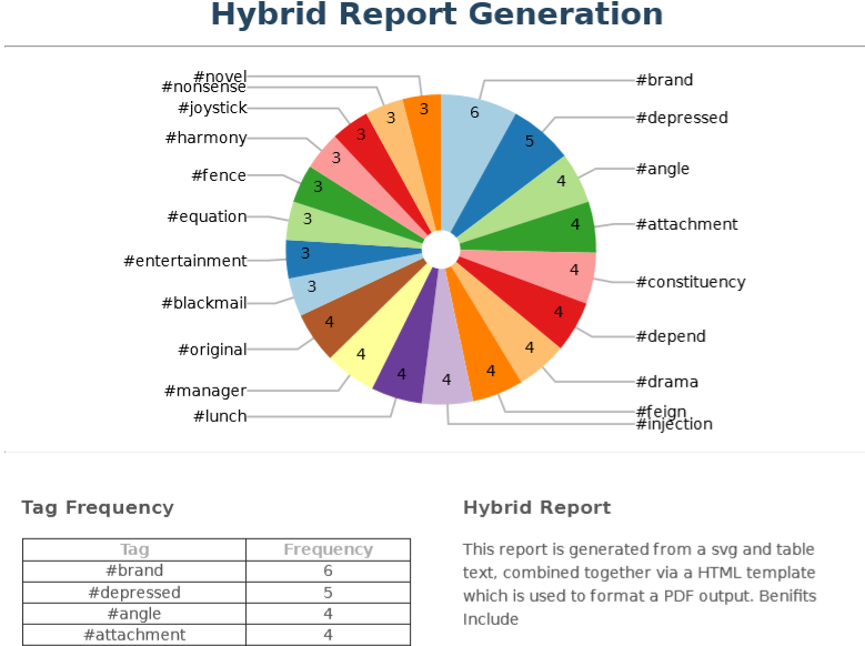 Using the method for SVG generation previously shown will combine it with text and other objects to create a complete document.
We will create an HTML document, laid out as we want the PDF to look, then convert the document into a PDF.
One of the advantages of using this method is the ability to use common CSS to ensure consistent styling.
To convert the HTML document to a PDF we will first render the HTML file in a fake browser and then export it as a PDF. We will use library called Puppeteer.
One point of note when using Puppeteer in a Lambda function is that you can run into timeout issues if using the smallest amount of allocated memory. As Puppeteer can use a large amount of memory so increasing the assigned resources to the AWS Lambda function would be recommended. We tested with various memory allocations and compared against the average run times in order to find a sweet spot which gave the best cost to speed ratio. We ultimately chose to assign 1024MB to the Lambdas which keeps run times down while maintaining low costs.
Enhancing on the process to generate our images, the complete workflow of creating a PDF looks like this -
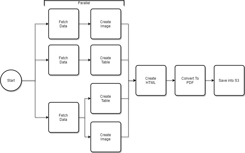
We can run each of the sections in parallel to improve processing time if there are multiple images or other PDF components which need to be created.
The processes used for image creation as the same as in the SVG example above. A full example can be found in this file, we will now cover each of the new sections in detail.
Create Table
To create tables or other data driven sections of HTML we can use standard Node.js functions to map over arrays to build our own HTML elements. This example builds table rows for the top y elements table.
	let tableinformation = '';
    tableData.forEach((item) => {
      tableinformation += `<tr><td>${item.key}</td><td>${item.doc_count}</td></tr>`;
    });
Create HTML
To build the HTML object which will be converted, we have a template file into which we pass in the relevant data we wish to display -
	module.exports = ({ svgData = '', textInformation = '', tableinformation = '' }) => {
      return `
        <html>
          <head>
              <title>Title Test</title>
              <style>
               /* CSS Stylings */
              </style>
          </head>
          <body>
              <h1>Hybrid Report Generation</h1>
              <hr />
              <div class="svgDiv">
                  ${svgData}
              </div>
              <hr />
              <div class="page-content">
              <div class="page-content-col page-content-col-left">
                  <h3>Tag Frequency</h3>
                  <table class="page-content-frequency-table">
                  <thead>
                      <tr>
                          <th>Tag</th>
                          <th>Frequency</th>
                      </tr>
                  </thead>
                  <tbody>
                      ${tableinformation}
                  </tbody>
                  </table>
              </div>
              <div class="page-content-col page-content-col-right">
                  <h3>Hybrid Report</h3>
                  <p>
                      Static Text
                  </p>
                  <p>
                      ${textInformation}
                  </p>
              </div>
              </div>
          </body>
        </html>
        `;
    };
As this generates HTML if we do not wish to convert to a PDF we could use this object for other purposes, such as creating email bodies or static webpages.
Convert to PDF
The process of creating the PDF uses the Puppeteer library which takes the formatted HTML we have produced and then converts it to a buffer -
    static async buildPDF({ formattedHTML = '' }) {
      const browser = await puppeteer.launch({
        args: chrome.args,
        executablePath: await chrome.executablePath,
        headless: chrome.headless,
      });
      const page = await browser.newPage();

      await page.setContent(formattedHTML);
      const buffer = await page.pdf({
        format: 'A4'
      });
      browser.close();

      return buffer;
    }
The process of converting to PDF is the most memory intensive part of the entire process, this is the key reason why we increase the available memory to the process. We must be careful to await on the setContent process to be finished before attempting to output the buffer, else we will end up with an empty PDF file produced.
Save into S3
To allow for the file to be downloaded and viewed, we need to save the buffer to an S3 bucket -
    async writeBufferToS3() {
		const s3 = new S3();
        const filename = `${uuidv4()}.pdf`;

        await s3.putObject({
          Bucket: this._bucketName,
          Key: filename,
          ContentType: 'application/pdf',
          ContentDisposition: 'download; fileName="Report.pdf"',
          Body: this._reportBuffer,
          Expires: fileTimeout()
        }).promise();

        return s3.getSignedUrl('getObject', {
          Bucket: this._bucketName,
          Key: filename,
          Expires: signedUrlTimeout()
        });
  	}
The processes for saving with a signed URL is always the same and uses methods from within the aws-sdk.
Conclusion
Generating these reports manually is laborious and is hard to keep consistency, by creating all reports within a central location we can keep them consistent. By moving as much of the process away from the user we can maintain control over the data presented. The pros and cons of this approach are -
Pros
- Obfuscate the raw data from a user. They only see the finished result.
- Frees client resources. Generating an SVG/PDF with lots of data will always be slower than viewing a pre-generated version.
- The viewing client does not need JavaScript enabled. This increases the places they can be used to include, for example emails.
- The finished file can be used for multiple purposes, such as emails.
- Use standard CSS formatting and styling.
Cons
- Run time of function when processing large data sets.