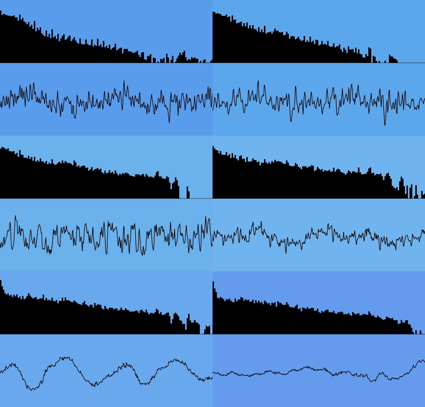
HTML5 adds a lot of new features for developers to make use of to build rich web applications. One of these is the Web Audio API – not to be confused with just the <audio> element – which allows access to raw audio data. This data can then be analysed and visualised through the HTML5 canvas or using charting libraries like D3.

You can see the application on GitHub Pages

Web Audio: What is it?

The Web Audio API (in brief) is a set of nodes connected together. These nodes can create, modify or output the audio. A rather basic analogy for this is the flow of water from a treatment plant to a house. The plant sends water (audio) though pipes, where it gets filtered and inspected, before being sent to the house (speakers) for use.

There’s a variety of ways audio can be created: by the CPU using an OscillatorNode; or from a file using AudioBufferSourceNode or the <audio> or <video> elements (MediaElementAudioSourceNode). The latter is especially powerful, as you can use real-time audio or video streams as a basis to do visualisation.

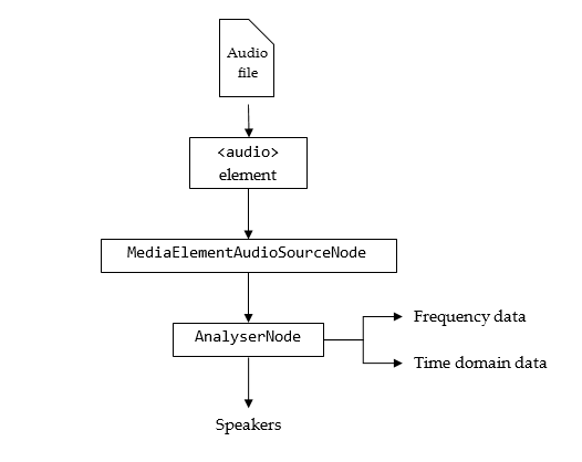
You can modify the audio data using a whole array of filters, such as high- or low-pass, delay and gain. I won’t touch on any of these in this post, however. The main magic used in this post is AnalyserNode, which provides a way to access frequency data and the data in the current time domain.

Central to the Web Audio API is the AudioContext. This provides a way to create these source and filter nodes, and eventually link them up with their destination – in this case, the speakers. One AudioContext is needed per audio stream (as the destination can only be from one node).

A more detailed description of the API can be found on MDN.

The Audio Pipeline

The audio pipeline needs to be set up in the correct way in order for us to visualise what’s going out to the speakers. If just an <audio> element was created, playing that would go straight to the speakers. So, a MediaElementAudioSourceNode is created with the element’s reference. That disconnects that element from the speakers, allowing code to reroute the audio through the Web Audio API.

The pipeline for the audio in this project is pretty straightforward. The MediaElementAudioSourceNode is linked to an AnalyserNode (where audio data is extracted for visualisation), which is then linked to the speakers.

For ease of use, the user drags and drops the audio files they wish to play onto the page (HTML5 Rocks has a guide to show how this is done). After they’ve done that, an <audio> element is created, and its source is set using an Object URL, which in this case acts like a remote URL but references a file or blob object.

var audioElement = document.createElement('audio');
audioElement.src = URL.createObjectURL(file); // eg. blob:http%3A//127.0.0.1%3A8080/af643450-98a6-4eac-aa87-ea9347ee007b

With the element created, the audio would play to the speakers straight away if it started playing. So, an AudioContext and MediaElementAudioSourceNode are created as follows:

var ctx = new AudioContext();
var sourceNode = ctx.createMediaElementSource(audioElement);

The AudioContext is needed as it is the basis for creating the audio nodes, and is also the nodes’ eventual destination. After the AnalyserNode has been made, it can just be connected to the speakers, represented by the AudioContext’s destination attribute.

var analyser = ctx.createAnalyser();
sourceNode.connect(analyser);
analyser.connect(ctx.destination);

And that’s all there is to setting up the audio pipeline – calling audioElement.play() will route the audio from the source node to the analyser, which passes it to the speakers.

Getting the Data from the Analyser

The AnalyserNode has a couple of functions that are being used – getFloatTimeDomainData and getFloatFrequencyData. These require the typed Float32Array, which helps keep things speedy. There’s also similar functions for Uint8Arrays.

getFloatTimeDomainData gets the current waveform being played, and is used as follows:

var array = new Float32Array(analyser.fftSize);
analyser.getFloatTimeDomainData(array);

which populates the typed array with the data. analyser.fftSize is a constant which denotes the size of the Fast Fourier Transform used in the creation of the waveform, which is the maximum number of data points which will be copied into the typed array.

getFloatFrequencyData works in a similar way, but analyser.fftSize is replaced by analyser.frequencyBinCount, which is the number of bins the frequencies are put into. frequencyBinCount is usually roughly half of the fftSize.

Bringing in D3

D3 is a library for performing SVG operations, and is well known for creating charts. The <svg> element is scaled to the browser’s size on page load and resize, and each different visualisation is scaled and positioned appropriately. In addition, drawing is repeated and throttled using requestAnimationFrame in order for it to as smoothly as possible in real-time. You can see the application in action on this GitHub Pages link.

Waveform

The waveform is most commonly expressed as a line, which is fairly simple to implement in terms of D3. The time domain data from the analyser is in the range [-1, 1], and so is straightforward to represent using two D3 scales.

var xScale = d3.scale.linear()
    .range([0, width])
    .domain([0, fftSize]);

var yScale = d3.scale.linear()
    .range([height, 0])
    .domain([-1, 1]);

var line = d3.svg.line()
    .x(function(d, i) { return xScale(i); })
    .y(function(d, i) { return yScale(d); });

selector.select("path")
    .datum(waveformData)
    .attr("d", line);

This works pretty well – there’s only one element in the DOM that is being changed, so the costliest part is the redraw. This cost was further reduced by subsampling the waveform to only draw width / 2 points, making the draw cheaper.

Frequency

The frequency data is a tad more complex, as that’s commonly represented as a set of rectangles. It doesn’t make much sense to draw each frequency bin – usually the bin count is 1024. Even with a 1080p display, that leaves less than 2 pixels per bin. So, the number of bars displayed is proportional to the width of the browser, and the frequency data is then put into a reduced number of bins using a basic average reduction:

function aggregate(data) {
    var aggregated = new Float32Array(numberOfBars);

    for(var i = 0; i < numberOfBars; i++) {
        var lowerBound = Math.floor(i / numberOfBars * data.length);
        var upperBound = Math.floor((i + 1) / numberOfBars * data.length);
        var bucket = data.slice(lowerBound, upperBound);

        aggregated[i] = bucket.reduce(function(acc, d) {
            return acc + d;
        }, 0) / bucket.length;
    }

    return aggregated;
}

The scales are much the same as before, with the exception that the domain on the Y scale is [-128, 0]. The actual domain goes below this, but most of the time the frequency levels do not reach that low unless the audio has finished. Anything under -128 can be background noise.

When all the rectangles are added (on the first frame draw or on resize), they are positioned and sized appropriately, based off of their index and the width per bar.

rect.enter()
    .append("rect")
    .attr("x", function(d, i) {
        return xScale(i);
    })
    .attr("width", function() {
        return selector.attr("width") / numberOfBars;
    })
    .attr("y", 0)
    .attr("class", "frequency-bar");

Note how the Y origin is set to 0. Normally, this would mean the bar starts on the top of the container and drops down. However, applying a transform: scaleY(-1) would cause this to flip the right way up for our needs, reducing the amount of DOM changes per frame – all that needs to be changed is the height.

When considering the height, the actual computation is a tiny bit more complicated, because we’re trimming -256 to -200 – if the height reaches below that, then it needs to be set to 1 to avoid errors and as a base case. The rectangles are also repositioned such that it remains on the bottom of its container.

    rect.attr("height", function(d) {
        var rectHeight = yScale(d);
        return rectHeight > 1 ? rectHeight : 1;
    });

This is just another simple bar chart-like component, tailored for the use of audio. In terms of performance, it’s a bit more of a hit here because hundreds of DOM elements are changed each frame (up to 60fps), each needing a redraw.

Coloured Background

An interesting idea was to try and represent the audio as a colour. The waveform could be used, but this is far too changeable from frame to frame. This wouldn’t necessarily be a problem if the waveform history was kept over a short period of time, but is more overhead for little gain. Instead, the frequency data was used, because that is smoothed over time (indeed, the AnalyserNode has a smoothingTimeConstant which determines how quickly it decays).

The approach used was to average different parts of the frequency spectrum to produce one number for each of the three colour dimensions. Using the Hue-Saturation-Lightness (HSL) spectrum seemed the most appropriate here, because it allows looking at different parts of the frequency spectrum to focus on different aspects of the colour, rather than the colour itself (which would have complicated an Red-Green-Blue based solution).

The hue dimension, which specifies the overall colour, was a simple average of the lower third of the spectrum. This was chosen because higher frequencies tend to have lower occurrence, and wouldn’t necessarily translate well into a representation of the file over time. Lightness, which signifies how dark or light the colour is, was an average over the entire spectrum in order to keep things faded and more constant than just the highly changeable lower frequencies. The saturation, which specifies how intense the colour is, was the average of the lower three frequency bins – the more intense the audio data, the more intense the colour produced.

After the averaging was done, colour was applied using D3 linear scales, as it allowed to specify the input and output domains. Hues are degrees (the HSL space is represented as a cylinder), whereas saturation and lightness are percentages. The range of these scales are smaller than the entire range available to use, in order to keep strobe effects to a minimum. The core of the code is as follows:

var scale = d3.scale.linear()
    .range([20, 90])
    .domain([-256, 0]);
var hueScale = d3.scale.linear()
    .range([250, 200])
    .domain([-120, -50]);

var h = reduceArray(data.slice(0, Math.floor(data.length / 3)));
var s = reduceArray(data.slice(0, 3));
var l = reduceArray(data.slice(data));

selector.select("rect")
    .attr("fill", "hsl(" + (hueScale(h)) + ", "
        + scale(s) + "%,"
        + scale(l) + "%)");

That’s It

That pretty much wraps up the nitty-gritty of using the Audio API with D3, and it’s straightforward due to the AnalyserNode being able to access audio data. I’ve thrown together a more complete application that also has a play queue and some text to go along with it, written using KnockoutJS and RequireJS. You can try this out on GitHub Pages with the code also being available on GitHub.