In my previous post, I created a fairly simple particle simulation where particles obey gravity, bouncing around in a box. This was a great way to get started with a non-trivial Go application. However, as the the particles didn’t interact with each other, there was limited potential for the simulation as a whole. In this post, I look at building on this simulation with another where particles obey forces of repulsion (and attraction).

Creating the Forces of Repulsion

In the previous post, the formula for determining the velocity of a particle was fairly straightforward: leave the X and Z components constant and and add a constant value to the Y component. This worked as it meant as the particles were leaving the ‘floor’ of the cube, the Y component of the velocity would be negative, and would so get smaller. When the particles peaked, they Y component would enter positive values and so would accelerate to the floor.

The base formula chosen to measure the forces of repulsion between particles was Coulomb’s Law. The particles would mainly have the same charge, so the formula essentially boils down to force = 1 / (distance between particles squared).

The function to perform this calculation was implemented at the particle level, where it was given a slice of other particles:

func (p *Particle) Tick(duration float64, otherParticles *[]Particle) {
    for _, otherParticle := range *otherParticles {
        // Get differences in x, y, z axis.
        xDiff, yDiff, zDiff := p.Position.X-otherParticle.Position.X,
            p.Position.Y-otherParticle.Position.Y,
            p.Position.Z-otherParticle.Position.Z

        // Combine the magnitudes of the differences together so that it can be used to divide up
        // the portions of the calculated force into the x, y, and z components
        combinedDifferences := math.Abs(xDiff) + math.Abs(yDiff) + math.Abs(zDiff)

        // Calculate the magnitude of the force between the two particles
        // k is some constant (defined here as 1)
        force := k / (math.Pow(xDiff, 2) + math.Pow(yDiff, 2) + math.Pow(zDiff, 2))

        // Normalise the force into the x, y, and z components.
        p.Vector.X += force * xDiff / combinedDifferences
        p.Vector.Y += force * yDiff / combinedDifferences
        p.Vector.Z += force * zDiff / combinedDifferences
    }

    // Update position using final velocities
    p.Position.X += duration * p.Vector.X
    p.Position.Y += duration * p.Vector.Y
    p.Position.Z += duration * p.Vector.Z
}

Having to calculate distance between potentially thousands of other points many thousands of times becomes quite an expensive operation. Therefore, finding a way to parallelise this becomes rather important.

Running in Parallel

The gravity approach in the previous post was great for parallelisation as the particles didn’t interact with each other, and as a result parallelisation was easy: allocate certain particles on each thread. For attraction and repulsion, the particles’ positions to each other determine the force acting upon it. Although the previous approach would work, would mean each thread would need every particle’s positions as well as which particles need to be updated, which would have large overheads both computationally and in memory footprint.

As previously mentioned, the formula is essentially force = 1 / (distance between particles squared). If that were to be plotted on a chart, it would look like:

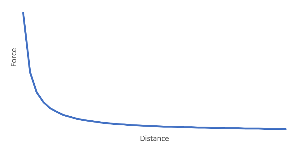
As can be seen, the line tends towards 0 with higher distance. Therefore, particles very far away would have a very minor (almost negligible) effect on the velocities. These particles can be discarded from a particular particle’s calculations.

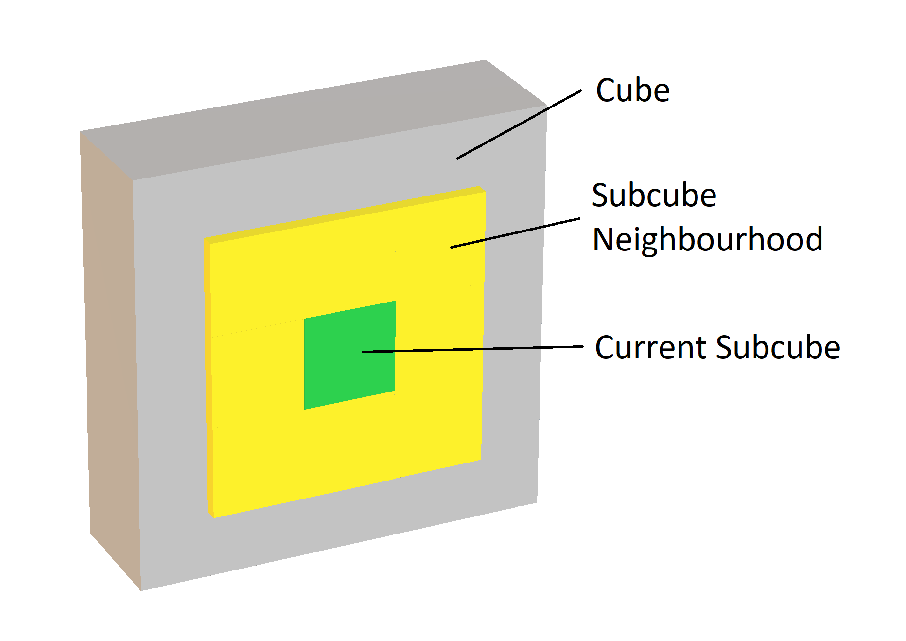
The way I approached this was dividing the cube where particles are bound into smaller “subcubes”. Each subcube represents all particles within a given volume of the larger cube. When calculating the forces acting upon each particle, all particles within that cube and a certain number of neighbouring cubes were assessed. The below image may help:

Dividing the particles this way means that not all of the particles are passed to each thread, meaning an iteration is cheaper and faster.

It’s worth mentioning that this approach will create a simulation that is similar but not identical to comparing each particle against each other. This is because the forces between all of the ignored particles would add up for each iteration, and so positions may be increasingly different per iteration.

During an iteration, the main thread sends the set of subcubes to each child thread (goroutine), then waits for the resulting positions returned by the goroutines. The goroutines are therefore relatively stateless and lightweight:

type inputChannel chan [][]primitives.Subcube
type outputChannel chan []primitives.Particle

// A thread that takes some input, ticks the particles, then returns some output.
func startSimulationThread(input inputChannel, output outputChannel) {
    var subcubes [][]primitives.Subcube
    ok := true
    for ok {
        // Wait for input from the main thread.
        subcubes, ok = <-input

        // If the channel hasn't closed
        if ok {
            var newPositions []primitives.Particle

            // Update the positions of each subcube.
            // A pointer is returned from Subcube.Tick to reduce memory footprint from pass-by-value
            for y := range subcubes {
                for z := range subcubes[y] {
                    newPositions = append(newPositions, (*subcubes[y][z].Tick(UNIT_TIME))...)
                }
            }

            // Return the new positions via the output channel
            output <- newPositions
        }
    }
}

During an iteration, managing the goroutines is also straightforward:

type Simulation struct {
    inputChannels  []inputChannel
    outputChannels []outputChannel
}

func (s *Simulation) Tick(subcubes *primitives.Subcubes) []primitives.Particle {
    // Send a slice via each input channel, and the relevant goroutine will pick it up
    for i, slice := range subcubes.Cubes {
        s.inputChannels[i] <- slice
    }

    var nextParticles []primitives.Particle

    // Wait for data from each channel, and once received, append to the slice
    for _, channel := range s.outputChannels {
        nextParticles = append(nextParticles, (<-channel)...)
    }

    return nextParticles
}

After all the of the iterations have been completed, cleaning up the goroutines is as simple as closing the channels:

for i := range inputChannels {
    close(inputChannels[i])
    close(outputChannels[i])
}

As particles may cross subcube boundaries during an iteration, the results for each thread needed to be fed back to the main thread where some housekeeping was applied – saving the current state of the particles, then recalculating the particles in each subcube and the neighbourhood of relevant particles for each subcube. The code for subcube management is as follows:

func (s *Subcubes) UpdateParticlePositions(particles *[]Particle) {
    // Clear each subcube of particles
    s.clearCubes()
    s.Particles = *particles

    for i := range s.Particles {
        // Get the x, y, z indices of the subcube the particle is in through simple math.Floor operations.
        x, y, z := getIntendedSubcube(&s.Particles[i], s.subcubeAxisSize)
        intendedSubcube := &s.Cubes[x][y][z]

        // Add that particle to the subcube
        intendedSubcube.Particles = append(intendedSubcube.Particles, s.Particles[i])
    }

    s.updateNeighbouringParticles()
}

// Iterates through all the subcubes, updating their relevant particles.
func (s *Subcubes) updateNeighbouringParticles() {
    for x := range s.Cubes {
        for y := range s.Cubes[x] {
            for z := range s.Cubes[x][y] {
                s.Cubes[x][y][z].RelevantParticles = *s.getNeighbouringParticles(x, y, z)
            }
        }
    }
}

func (s *Subcubes) getNeighbouringParticles(x, y, z int) *[]Particle {
    var particles []Particle
    CUBE_RANGE := 3
    CUBES_PER_AXIS := float64(len(s.Cubes))

    // Calculate the start and end indices for each axis, clamping them as required.
    // +1 for end indices to make them inclusive when slicing
    startX := int(math.Max(0.0, math.Min(float64(x-CUBE_RANGE), CUBES_PER_AXIS)))
    endX := int(math.Max(0.0, math.Min(float64(x+CUBE_RANGE+1), CUBES_PER_AXIS)))
    startY := int(math.Max(0.0, math.Min(float64(y-CUBE_RANGE), CUBES_PER_AXIS)))
    endY := int(math.Max(0.0, math.Min(float64(y+CUBE_RANGE+1), CUBES_PER_AXIS)))
    startZ := int(math.Max(0.0, math.Min(float64(z-CUBE_RANGE), CUBES_PER_AXIS)))
    endZ := int(math.Max(0.0, math.Min(float64(z+CUBE_RANGE+1), CUBES_PER_AXIS)))

    // For each subcube within the cube range, add all the particles
    for xIndex := range s.Cubes[startX:endX] {
        yZSlice := s.Cubes[startX+xIndex]

        for yIndex := range yZSlice[startY:endY] {
            zSlice := yZSlice[startY+yIndex]

            for _, subcube := range zSlice[startZ:endZ] {
                particles = append(particles, subcube.Particles...)
            }
        }
    }

    return &particles
}

The Results

A large number of particles were needed to create a visualisation and to showcase performance improvements. As the radius calculations were the most expensive part of the calculations, increasing the number of subcubes improved performance up to a certain point. Then, the cost of maintaining the subcubes exceeded the amount of time doing the position calculations.

As a result of the above optimisations, the following video was created. In it, 10,000 particles were simulated repelling each other over 500 iterations, with 40 x 40 x 40 subcubes (64,000 total). The total calculation time was 4 minutes – 50 frames of the video took approximately 24 seconds to produce. On a single-threaded implementation, 50 frames took multiple minutes with just 5000 particles.

Creating the Visualisations

The Go programme itself was rather simple in that it didn’t produce any visualisations. Instead, it created a CSV file per unit time of the simulation. These CSV files had one particle per row, with the X, Y, and Z co-ordinates being the row data.

The series of CSV files were fed into ParaView using the Table To Points filter, and then exported to a video file.

The programme could be expanded to perform the visualisation, perhaps using OpenGL bindings.

Wrapping Up

All in all, I was very impressed at the results the simulation produced. Initially, you can see patterns in the particles’ locations due to the subcube method, though increasing the radius of other subcubes to consider would improve this. The performance improved markedly as a result of the parallelisation approach. The approach is one that fits rather well in this case - short range repulsion, with an exponential tail off in force values. Using other formulae for simulations may require a some changes to the approach.

As ever, the code for the simulation is available on GitHub.