Back in September last year, the Guardian published a fantastic visualisation looking at house price affordability in the United Kingdom. They took the Prices Paid data from the Land Registry and computed some descriptive statistics about it, such as the median and range.

The raw data is easily available from data.gov.uk, and they provide monthly, annual and the complete history allowing you to work with a reasonably sized set before running on the complete data set.

Recreating the Guardian’s data process within Apache Spark felt like a great way to get an introduction into the platform.

What Is Apache Spark

Spark is one of the most common platforms used for large scale data processing today. It builds upon the MapReduce programming model introduced by Hadoop. However, It is significantly faster than Hadoop (up to 100 times) as it performs the operations in memory avoiding slow disk IO operations.

It is a general-purpose platform. You can clean, process and analyse data all within Spark. It has connectivity to various data storage platforms and can cope with either structured (for example SQL data via JDBC) or unstructured data stored (such as text files in HDFS). It is designed to cope with large scale data, way beyond what can be stored within a single machine capabilities. It integrates with Hadoop easily and can use Hadoop’s YARN system to find and control computation nodes in the network.

There is support for Java, Scala, Python and R. This means you can quickly get up and started if you have familiarity in any of these languages. For all but Java, there is also a REPL style environment. In this post, I will be looking at using Python with Spark and using a Jupyter notebook as an interactive environment to experiment with the data, but all of the commands are common across the different languages.

Spark has two ways of looking at data at each node. Either as an RDD (Resilient Distributed Datasets) or a DataFrame. For this post, I am only looking at RDDs. An RDD is a fundamental data structure of Spark. It is an immutable, partitioned set of data. It can contain a set of any Java, Scala or Python objects (including custom classes). They contain the lineage of the data (the steps used to create them), so are resilient as they can be easily recreated. An RDD can either be a basic table of objects or can be a set of key and value pairs. There are some special functions for working with key based RDDs which provide great functionality and power (e.g. reduceByKey and groupByKey).

The lineage also allows for lazy evaluation, in other words nothing is evaluated until a result is needed. Spark handles this by having two types of functions - Transformations and Actions. Transformations do not cause the evaluation of an RDD but instead reshape the input RDD to a new RDD. A simple example of a transformation would be a map extracting a couple of values or a filter selecting a subset of rows. Actions cause the RDD to be evaluated and return a result. A simple example would be the count function which returns the number of rows in the RDD. One interesting thing is the while reduce is itself an action returning a single item, but reduceByKey is a transformation returning a new RDD of keys and values.

The Map Reduce model

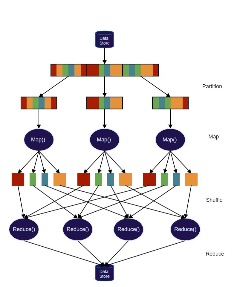
The first part of the process is ‘ingesting’ the data from a data store. This data is then partitioned and passed into different computation nodes to process. If you take the simple case of reading a flat file from the filesystem, this means just reading in multiple blocks.

These partitioned blocks of data then go through the ‘map’ part of the process. This layer might do things like filtering the data, restructuring the data or sorting the data. Following this, the resulting mapped data may need to be redistributed between nodes to allow for the next stage of the computation. This ‘shuffle’ of the data is the slowest part of the process as it involved data leaving one node and moving to another, which will generally be a different computer.

The final stage in the MapReduce process is to ‘reduce’ the data to produce a useful result set. These are summary operations such counting number of records or computing averages. The reduce process can be multiple layers with nodes computing intermediary results before passing them on to be aggregated to produce the final result set.

Installing Spark

First, we need to install some pre-requisites. Spark itself needs a Java VM to run, you can download the current version from the Java home page. We will be using Python for this tutorial. I chose to use version 3.x, but everything works in 2.x as well. In order to use a Jupyter notebook as a development environment, you also need to install that. I chose to use the Anaconda Python distribution which includes everything I needed (including the notebooks).

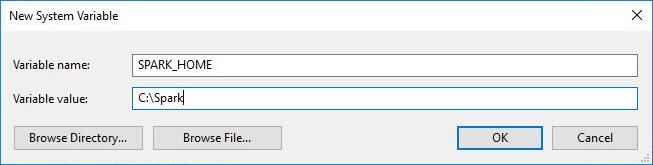
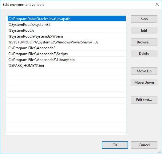
For this guide, we won’t be using Hadoop and will just be running a local instance of Spark. You can hence download whichever version of Spark you like from the download page. Once you have downloaded it, extract the file to a location you are happy to run it from, I used C:\Spark. We now need to set up some environment variables. First, add a new environment variable called SPARK_HOME and set it to the location you extracted Spark to. Next, add %SPARK_HOME%\bin to the Path variable.

If you have both Python 2 and 3 installed on the same machine, you will need to tell Spark to use Python 3. This can be done by another environment variable PYSPARK_DRIVER and setting it to the command to run Python 3 (e.g. SET PYSPARK_DRIVER=python3).

To run on Windows, we need to resolve an issue to do with a permission error for Hive. To fix this:

• Download winutils.exe and save it to somewhere like C:\Hadoop\bin.
• Create a new environment variable HADOOP_HOME pointing at C:\Hadoop.
• Add an entry to the Path variable equal to %HADOOP_HOME%\bin.
• Make a new directory C:\Tmp\Hive.
• In a console window run winutil chmod -R 777 \Tmp\Hive.

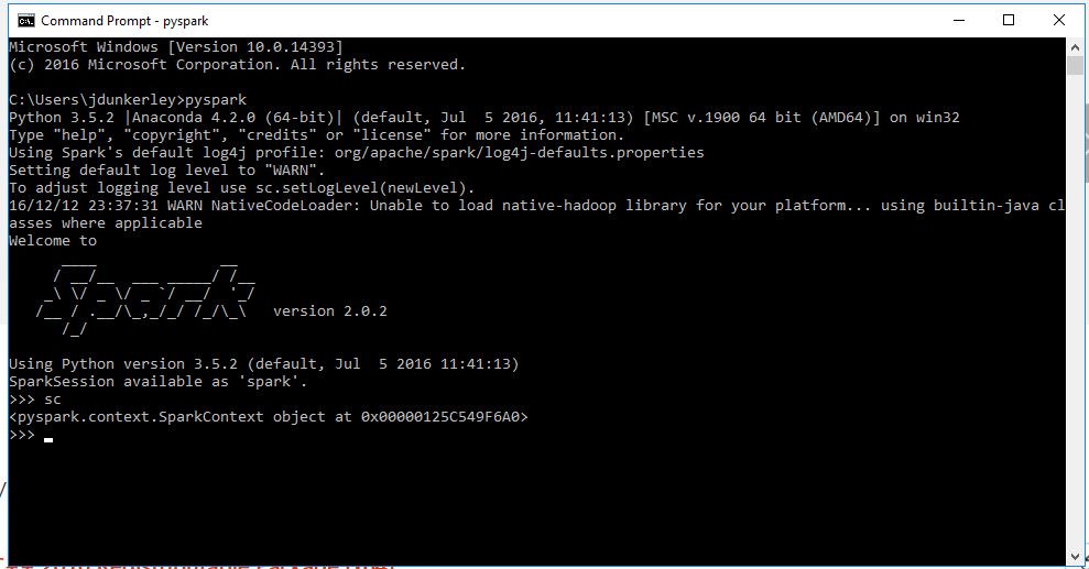
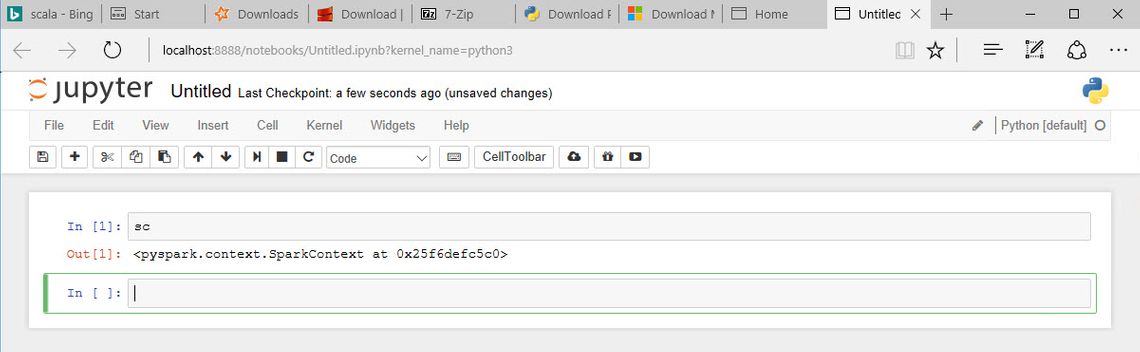
Now to test we are all set up. Open a new console window and enter the command pyspark. This should launch a new Python based Spark console session. We can type sc in and check that the variable has been set to a Spark Context:

Finally, we now want to tell Spark to use the Jupyter notebook so we can experiment. To do this we need to set two more environment variables. The first PYSPARK_DRIVER_PYTHON should be set to jupyter to tell Spark to run the notebook command. The second PYSPARK_DRIVER_PYTHON_OPTS needs to be set notebook. Now if we run pyspark, we will get an interactive notebook session in a browser:

While the instructions above are based on a Windows process, the same instructions will configure a Mac to run it as well. You shouldn’t remove python 2.x! You will need to add the environment variables to ~./bashrc file:

EXPORT SPARK_HOME = /usr/local/spark
EXPORT PATH = $PATH:/usr/local/spark/bin
EXPORT PYSPARK_DRIVER = python3
EXPORT PYSPARK_DRIVER_PYTHON = jupyter
EXPORT PYSPARK_DRIVER_PYTHON_OPTS = notebook

Reading and Parsing the Raw Data

The data file from the Land Registry is just a plain CSV file:

"{3E0330EF-67CA-8D89-E050-A8C062052140}","112000","2006-05-22 00:00","MK13 7QS","F","N","L","HOME RIDINGS HOUSE","13","FLINTERGILL COURT","HEELANDS","MILTON KEYNES","MILTON KEYNES","MILTON KEYNES","A","A"
"{3E0330EF-7707-8D89-E050-A8C062052140}","900000","2006-06-29 00:00","CH3 7QN","S","N","F","CHURCH MANOR","","VILLAGE ROAD","WAVERTON","CHESTER","CHESHIRE WEST AND CHESTER","CHESHIRE WEST AND CHESTER","A","A"
"{3E0330EF-A324-8D89-E050-A8C062052140}","250000","2006-07-07 00:00","DE6 3DE","T","N","F","DALE ABBEY HOUSE","","","LONGFORD","ASHBOURNE","DERBYSHIRE DALES","DERBYSHIRE","A","A"
"{3E0330EF-BF0B-8D89-E050-A8C062052140}","157000","2006-12-01 00:00","M25 1HF","T","N","F","9A","","HEATON STREET","PRESTWICH","MANCHESTER","BURY","GREATER MANCHESTER","A","A"
"{3E0330F0-16DA-8D89-E050-A8C062052140}","326500","2006-11-24 00:00","SW6 1LJ","F","N","L","60","","ANSELM ROAD","","LONDON","HAMMERSMITH AND FULHAM","GREATER LONDON","A","A"
...

Each field in the file is stored as a text value surrounded by quotes. They also don’t store the header in the files but details can be found in the details provided. The first task is to read the raw text file into an RDD. This is very straight forward using sc.textFile(FileName) and we can then verify the content by checking the first 5 lines using take(5). It is worth noting that prior to calling take, Spark won’t actually have done any work.

For each line in the text file, we want to break it into an array of value and then convert from this to a dictionary attaching a header. The small script below shows one way to do this using the map function combined with Python lambda functions:

header = ['Transaction unique identifier','Price','Date of Transfer','Postcode','Property Type','Old/New','Duration', \
          'PAON','SAON','Street','Locality','Town/City','District','County','PPDCategory Type']

data = sc.textFile(r'C:\Downloads\pp-monthly-update-new-version.csv') \
    .map(lambda line: line.strip('"').split('","')) \
    .map(lambda array: dict(zip(header, array)))

data.take(5)

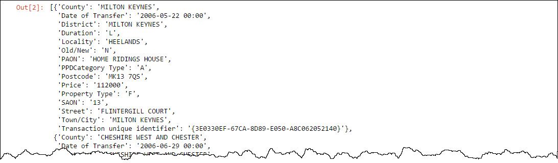
I only want to deal with the ‘outward code’ part of the Postcode (i.e. the part before the space) and for simplicity at this stage I am going to remove records which don’t have a postcode. As the intention is to run this over the entire dataset from 1995, I will also need the year. As I only need the year, I can just read the first four characters of the date and avoid parsing into a Python date object. Finally, I want to create a key based RDD. All you need to do for this within Python in Spark is return tuples rather than values. I went for a simple (year)_(postcode) for the key, with the price as the value. The function for the data now becomes:

indexPostcode = 3
indexPrice = 1
indexDate = 2
data = sc.textFile(r'C:\Downloads\pp-monthly-update-new-version.csv')\
    .map(lambda line: line.strip('"').split('","'))\
    .filter(lambda d: d[indexPostcode] != '') \
    .map(lambda d: (d[indexDate][0:4] + '_' + d[indexPostcode].split(' ')[0], int(d[indexPrice])))

Computing the statistics

At this point, I have a dataset shaped how I want and with keys as I wanted. In other words, we have done the Map part of the process. I now wanted to look at some basic statistics. Taking a look first at the total count of all records and the counts by key. Unlike virtually all the other byKey methods, countByKey is itself an action returning a dictionary rather than an RDD. I also wanted to look at the range of the price. Computing the maximum and minimum value can easily be done using the reduceByKey transformation and the reading with an action such as collect (which gets all the values from the RDD) to see the values. The block of code below shows the calculation of these four statistics:

totalCount = data.count()
countsByKeyDict = data.countByKey()
maxByKey = data.reduceByKey(max)
minByKey = data.reduceByKey(min)

To compute the mean and standard deviation, you need to compute the total of all the values and the sum of prices squared. Again, this can be done using the reduceByKey but this time I need to provide a bespoke function to do the computation. Python lambda syntax is particularly suited to this simple computation. For the sum of the squared value, the map function is used to compute the squared value before running reduceByKey. Note that when using map with a keyed RDD, the function will be passed a tuple of the key and value. I also need to be able to interact with the counts, again this can be done using map and reduceByKey. Finally, to join the values together, you need to use join to look up one value from one RDD into another based on the key. Combined with map this can be used to compute the mean and standard deviation. The code below will create RDDs capable of producing all of the basic statistics:

import math
countByKey = data.map(lambda kvp: (kvp[0], 1)).reduceByKey(lambda a,b: a + b)
maxByKey = data.reduceByKey(max)
minByKey = data.reduceByKey(min)
totalByKey = data.reduceByKey(lambda a,b: a + b)
sumSqByKey = data.map(lambda kvp: (kvp[0], kvp[1]**2)).reduceByKey(lambda a,b: a + b)
mean = totalByKey.join(countByKey).map(lambda kvp: (kvp[0], kvp[1][0] / kvp[1][1]))
avgSquare = sumSqByKey.join(countByKey).map(lambda kvp: (kvp[0], kvp[1][0] / kvp[1][1]))
stDev = avgSquare.join(mean).map(lambda kvp: (kvp[0], math.sqrt(kvp[1][0] - kvp[1][1]**2)))

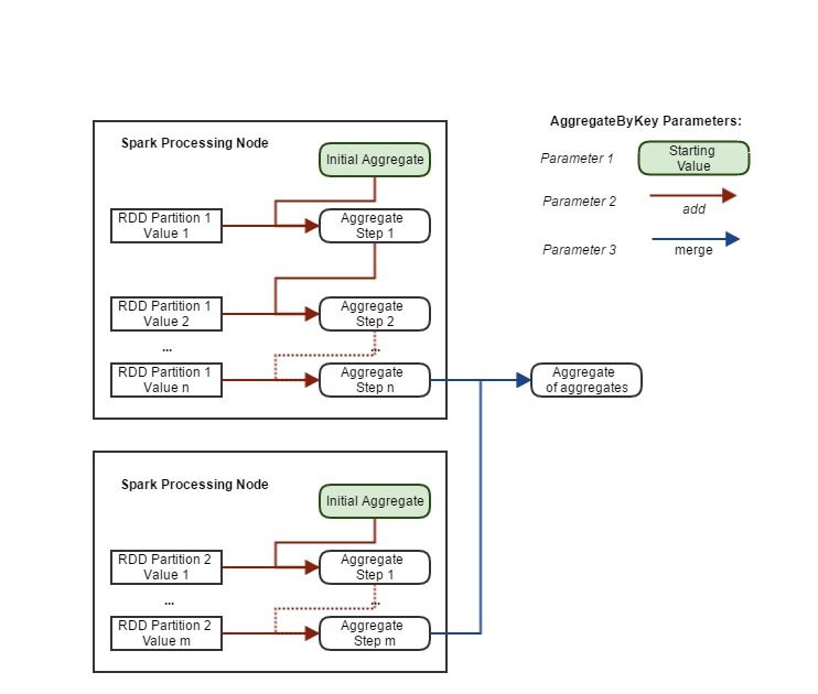
All of these statistics can be computed in a single pass together. We need to use the aggregateByKey function to do this. This function takes 3 parameters. The first is the value to initiate the aggregation process with. The second is a function argument which takes the current aggregate value (or the initial value) and a single value from the RDD and then computes the new value of the aggregate. For each key, this function is called for every value within a computation node to compute the aggregate value. If a key is split across multiple nodes, then this aggregate is passed to the final parameter. This is a function argument which takes two aggregate value and merges them. This will be called repeatedly until a final single aggregate for the key is computed. This final function will not be called for a key, if all of its values are within a single node.

As a simple example, the code below computes the mean of the price using aggregateByKey. As it moved down the RDD records within each key, it aggregates them into an array containing the count and the total. The mean is then computed from the final aggregate array for each key using a map function.

mean = data.aggregateByKey([0, 0],\
                            lambda c,v: [c[0] + 1, c[1] + v],\
                            lambda a,b: [a[0] + b[0], a[1] + b[1]])\
           .map(lambda kvp: (kvp[0], kvp[1][1] / kvp[1][0]))

For computing all of the statistics, I extend the above approach to be an array of 5 values: Count, Sum, Sum of Square, Max and Min. I find it cleaner to move away from the lambda syntax at this point and move to defining functions for each of the steps. The code below computes all of the above statistics and returns them as a dictionary:

import math

initialAggregate = [0, 0, 0, 10000000000, 0]

def addValue(current, value):
    return [
        current[0] + 1,
        current[1] + value,
        current[2] + value ** 2,
        min(current[3], value),
        max(current[4], value)]

def mergeAggregates(a, b):
    return [
        a[0] + b[0],
        a[1] + b[1],
        a[2] + b[2],
        min(a[3], b[3]),
        max(a[4], b[4])]

header = ['Count', 'Mean', 'StDev', 'Min', 'Max']
def aggregateToArray(a):
    return [a[0], a[1] / a[0], math.sqrt(a[2] / a[0] - (a[1] / a[0]) ** 2), a[3], a[4]]

stats = data.aggregateByKey(initialAggregate, addValue, mergeAggregates)\
           .map(lambda kvp: (kvp[0], dict(zip(header, aggregateToArray(kvp[1])))))

If you would rather use a Python class for this, there is a limitation that the PySpark cannot pickle a class in the main script file. If you place the implementation in a separate module, then you will be able to use it. While this is quite straight forward as a Spark Job, it is a restriction to work around within the REPL environment.

The final statistic I want to compute, is the median. While for very large datasets, we won’t be able to use a straight forward approach, the price paid data is small enough to use a simple groupByKey method. This method groups together all the values for a key into an array. We can then use the map function on the array to compute the median. The limitation of this approach is that it is possible you won’t be able to store all the values for a key in a single node in which case an out of memory exception will occur. It also requires a large amount of data being moved between the nodes. However, for this simple case the code looks like:

import statistics
medians = data.groupByKey()\
    .map(lambda kvp: (kvp[0], statistics.median(kvp[1])))

We now have all the statistics needed. The last task is to join it all back together and output the results. The join command easily allows us to join the median to the other statistics. In order to write it out to a CSV file, we need to join the partitions back together. We can use the repartition function to either increase or decrease the number of partitions. In this case I want to reduce to a single partition. The code below adds a header row, creates an array of values from the statistics and converts to a comma separated string, and finally writes to a CSV file within the specified folder (saveAsTextFile):

import copy
def mergeStats(dict, median):
    output = copy.copy(dict)
    output["Median"] = median
    return output

allStats = stats.join(medians).map(lambda kvp: (kvp[0], mergeStats(kvp[1][0], kvp[1][1])))

outputHeader = ['Count', 'Mean', 'StDev', 'Median', 'Min', 'Max']
csvData = allStats\
    .map(lambda kvp: kvp[0][0:4] + ',' + kvp[0][5:] + ',' + ",".join(map(str, map(lambda k: kvp[1][k], outputHeader))))

sc.parallelize(['Year,Postcode,' + ",".join(outputHeader)])\
    .union(csvData)\
    .repartition(1)\
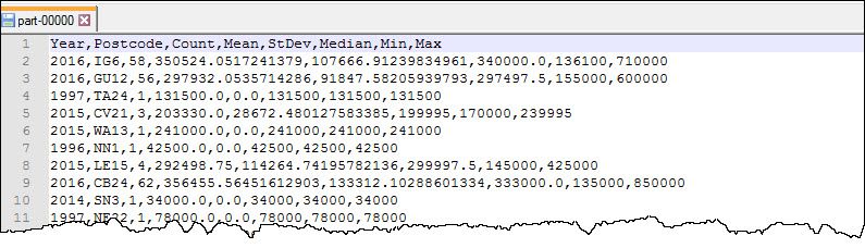
    .saveAsTextFile(r'C:\Downloads\pricePaidStatistics')

Running this process produces the output below:

Creating a Spark Job

To convert this from a REPL script to a Spark Job we can run needs a little wrapping. The code below will set up the Spark context and allow you to run it using spark-submit command:

from pyspark import SparkConf, SparkContext

def main(sc):
    #Insert Data Code Here

if __name__ == "__main__":
    conf = SparkConf().setAppName("APPNAME") # Update APPNAME
    conf = conf.setMaster("local[*]")
    sc = SparkContext(conf=conf)

    main(sc)

Once you have put together the complete script you can then run it at the command line. You need to unset the PYSPARK_DRIVER_PYTHON and the PYSPARK_DRIVER_PYTHON_OPTS before running the spark-submit command:

set PYSPARK_DRIVER_PYTHON=
set PYSPARK_DRIVER_PYTHON_OPTS=
spark-submit spark_pricesPaid.py

This will produce a lot of log messages:

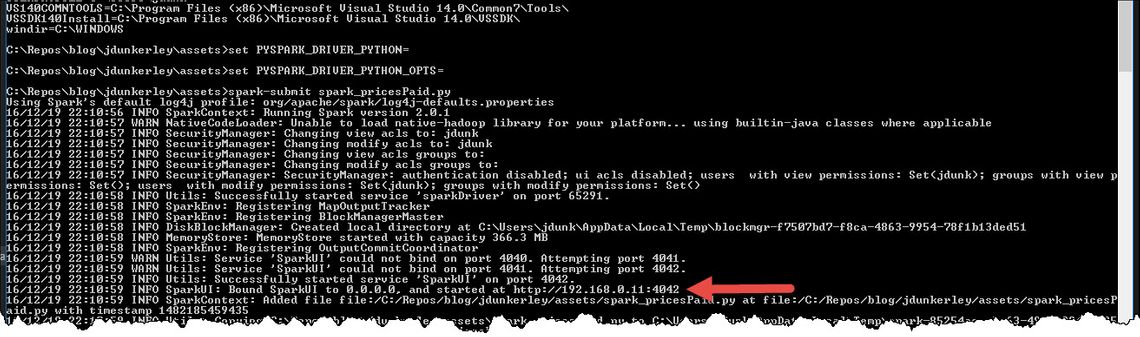
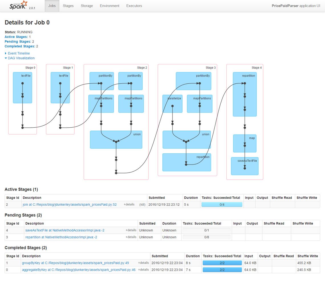
When you run a process within Spark, it automatically creates a web based UI you can use to monitor what is going. This is true in either the REPL environment or when running as a Spark job. The arrow shows the log message indicating the URL. It will be the first free port after 4040. It has some great features and is worth exploring. The screen shot below show the DAG for the process created in this post.

What Next

Hopefully this has given you a taste of the power of Spark. It is a fantastic platform for data analytics and has a huge community supporting it. There are extensions for Machine Learning and for Streaming. It is easy to get started and produce some results quickly.