Agile Progress and Quality Reporting
In the delivery space, a multitude of metrics have been used to express the state of product development. Many metrics we have seen traditionally are measuring some flavour of actual vs planned progress, often in terms of scope completeness per milestone or budget consumed vs scope achieved. In addition, quality is mostly perceived as some metric around bugs raised and fixed.
When making use of an agile approach we cannot rely on scope staying fixed according to a longer plan. Hence, scope related metrics fall significantly short of what we need to understand how well (or badly) product development is going. One of the tenets of agile is that ‘Working software is the primary measure of progress’ (see the principles attached to the manifesto). With this in mind, we can use Flow to judge our ability to produce working software and get it out to the user.
Measuring business value is important to ensure our progress is going in the right direction - that we produce the right outcomes. I have covered this topic in my recent post around business agility.
However, in addition to metrics for progress efficiency and business value, there is also the question of how to report on quality and what metrics to use. Hence, after going into Flow for efficiency I’d like to introduce a different approach to reporting quality than done in traditional projects.
In summary, there are three types of relevant metrics in agile product deliveries:
- metrics that focus on the creation of business value
- measuring efficiency of the delivery capability,
- metrics trying to describe quality.
Process Flow is the fundamental efficiency metric for agility
To get a feeling for what Flow is you can play the Ball Point Game, watch traffic or observe a small river with large stones in it. Process Flow is very similar in how it reacts to obstacles (stones in the river), overloading the system with work (put more and more cars on a road) or the effect of not having slack (the traffic movie earlier is showing what happens then).
In a well flowing system, items pass through the system without pause even if some stages of the process take more or less time than others. You can see the effect of different speeds in a system in a widening and narrowing river bed and watch the water vary its speed - it will never stop entirely unless you build a dam. The effect is that you can predict very well how much time it will take for an item to pass through. Without traffic jams, accidents and traffic lights it is easy to predict how long it will take from A to B using a given route.
When we achieve Flow in a system, individual items finish as quick as possible given the parameters of the system (e.g. skills and infrastructure) and by that Flow enables quick Build – Measure – Learn feedback loops. Rapid feedback loops are one of the foundations of empiricism and agility in any framework, e.g. Scrum or Kanban. Interestingly, those approaches address process Flow without being necessarily explicit about it. Scrum, for example, uses Sprints to force short feedback loops and DevOps looks at techniques to deliver into production quicker and more often.
Making Flow our guiding light provides a vision for meaningful improvements to a delivery capability, including looking at right-sizing User Stories, effective team-level communication and healthy burn-down charts.
Little’s Law
The key components describing Flow are
-
Cycle Time (CT) The amount of time to get a piece of work done, from start to finish.
-
Work in Progress (WIP) The number of work items in progress at a given time.
-
Throughput (TP) The number of work items finished during a time period.
Part of these metrics usefulness is that they can be easily explained to people at any level of seniority and they will make sense from each of their perspectives. They can be used for reporting upwards and for the team.
They are bound together by Little’s Law:1
\[\overline{CT} = \frac{\overline{WIP}}{\overline{TP}}\]The law makes the relation of the above metrics clear and gives us some powerful tools to understand how to improve Flow by using the assumptions of Little’s Law. But at the same time, it must be stated that Little’s Law is a law of averages and it is not usable to calculate values for individual items.
However, from the relationship stated in the law we can clearly see that cycle time can be shortened by either reducing work in progress or increasing throughput. The first can be achieved by work in progress limits as it is done in Kanban and the second by reducing item size. It also puts pairing as a practice in an interesting light, where we work on fewer items at any one time and get each individual item quicker through the system which reduces cycle time.2
Assumptions for predictability
- $\overline{\text{Arrival Rate}}$ = $\overline{\text{Departure Rate}}$
- All tasks will eventually exit the system
- No large variance in WIP
- $\overline{\text{WIP age}}$ constant
- Consistent units
These assumptions must be satisfied for Little’s Law to be applicable. We can use them to judge the predictability of a system. They help us guide our questions when analysing a delivery capability. They can also guide improvement efforts and enable us to measure efficiency and predictability improvements easily.
Analysing Flow with Cumulative Flow Diagrams
Cumulative Flow Diagrams (CFDs) are a great visual way to understand Flow in a system that helps us assuring Little’s Law assumptions and allows spotting potential problem states. It is often used in Kanban but is actually not limited to this approach. The input data are arrival and departure dates for each work item at each of their states in the process.
If for example, a process uses the states analysis, development and test we record arrival at each of those states, e.g. when did analysis start and the departure from the state, e.g. when was analysis done. All the items departed from the last stage are truly done and form the body of completed work.
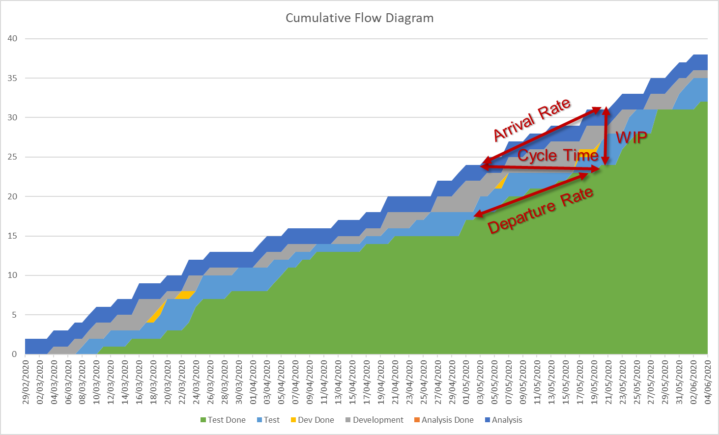
Example Cumulative Flow Diagram showing average arrival rate, estimated average cycle time, work in progress and average departure rate.
The first assumption of Little’s Law can be simply checked in a CFD by comparing the top slope and bottom slope of the graph. If they widen or narrow the first assumption is not fulfilled. If the width of each band in the CFD does not have a large variance, the third assumption is fulfilled. Problems with the second and fourth assumption are harder to spot in a CFD and need to be monitored specifically.
The data for CFDs are the start and end dates for each item and each stage. It can be easily recorded manually on a day to day basis or exported from electronic systems used for task tracking like JIRA or Azure DevOps.
Example problem states are indicated by
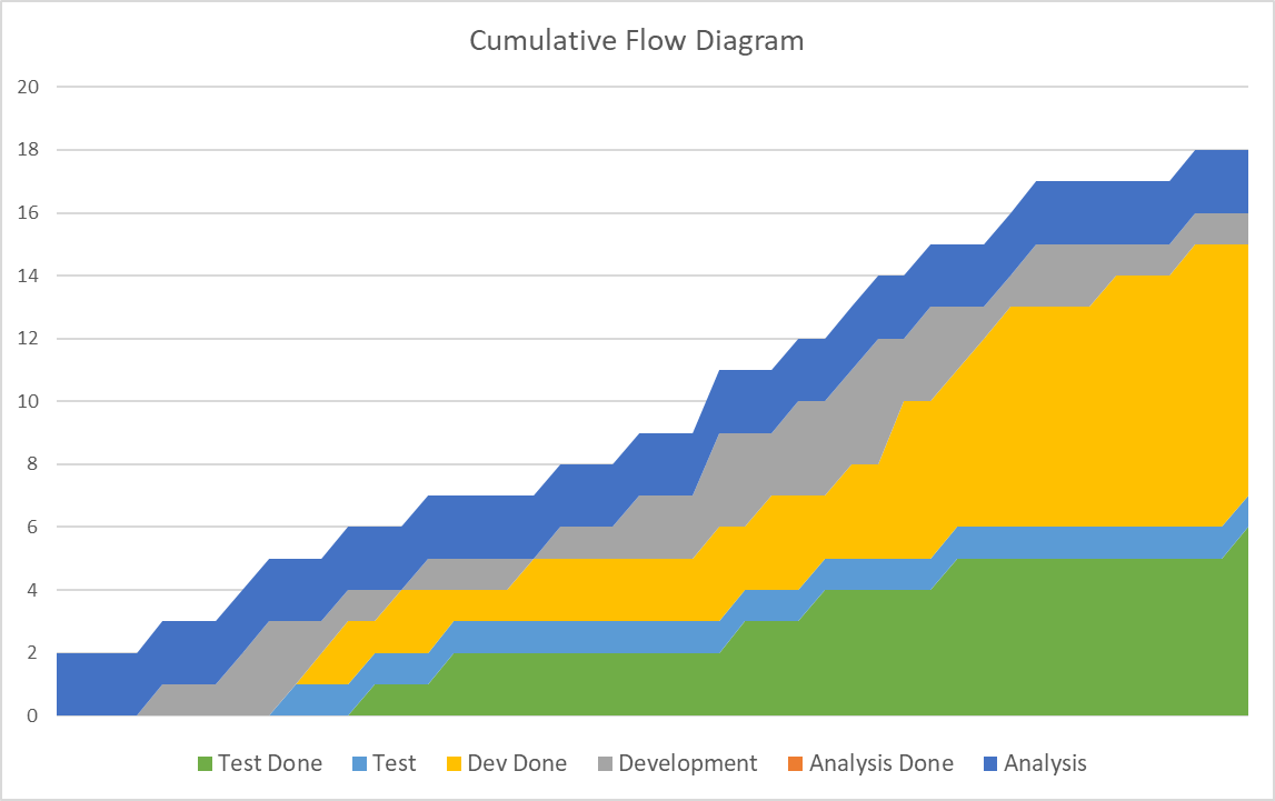
- Flat lines show that items are stuck between two states indicating an impediment causing waiting time (one of the wastes in Lean). This situation indicates increasing WIP age and a violation of the fourth assumption.
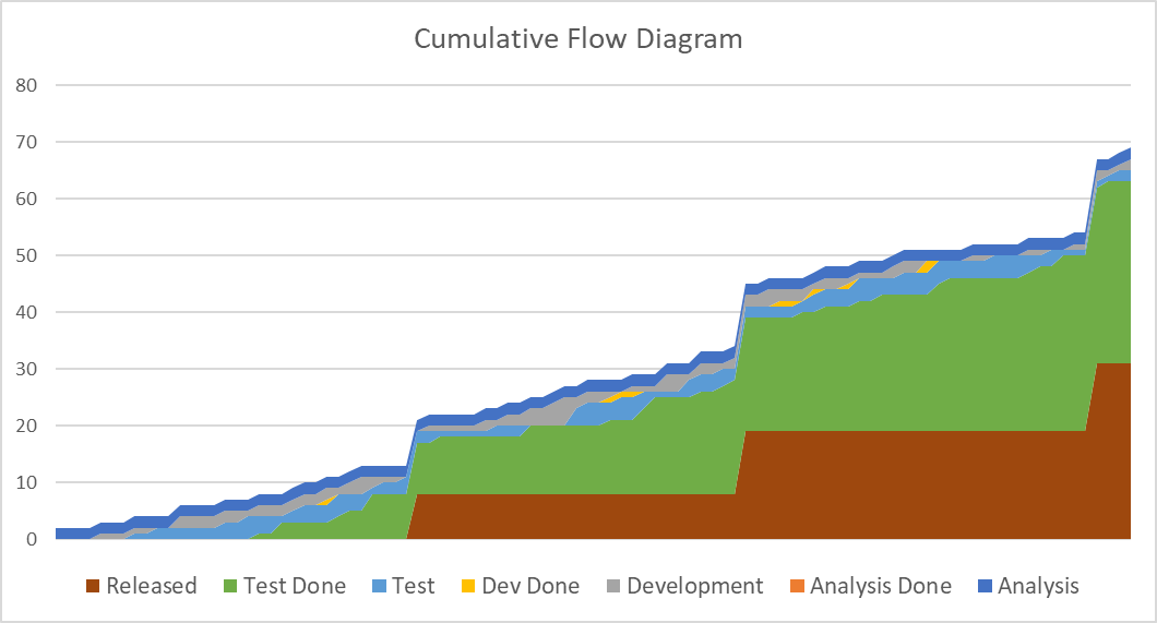
- Stair steps indicate delivery in batches with zero done work before release. While not necessarily a problem for Little’s Law it has its shortcomings in terms of time to market and the speed of the feedback loop. When using Scrum you will naturally see them if your definition of done includes release to users.
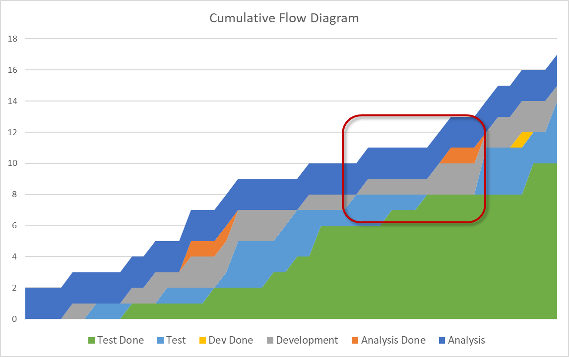
- Disappearing bands signify a drastic problem: a process step is starved for work items. This means an earlier process step is not delivering quick enough. Example reasons can be impediments or too little capacity in the earlier stages or too much capacity in the starved process step.

- Bulging bands are similar to disappearing bands: there is a bottleneck, in this case not in a preceding step but in following one.
Forecasting
Given a stable system in accordance with Little’s Law’s assumptions from above – percentiles in scatterplots (throughput on the y-axis, time on the x-axis, plot each done item’s cycle time) of cycle time yield a simple means for probabilistic forecasting of single items. The level of confidence can be used according to the risk appetite of the organisation. Communication involving probabilistic forecasting will naturally avoid the interpretation of guaranteed goalposts but instead clearly message that there is uncertainty and even quantify it.
Although cycle time scatterplots are useful only for forecasting a single item, you can choose yourself the complexity of the item. You can do it with tasks, User Stories or even Epics if you have the relevant data. It is, of course, important to keep the units consistent: if you want to forecast Epics you should plot Epics and if you are interested in User Stories plot those. What makes the approach very nice to use is that as long as you have a representative population the relative size of the type you plot does not matter and you don’t even need an estimate for the item you want to forecast.
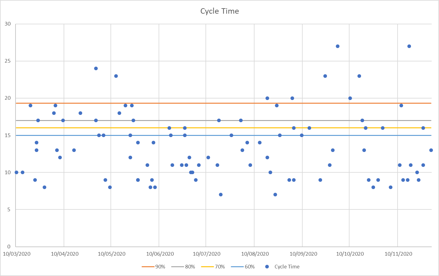
Plot of all done items with their cycle time on the day they were done. Horizontal lines are the percentiles at 60%, 70%, 80% and 90%. Note that the gap between percentiles is getting larger the higher the percentile. The 100% percentile would be at the level of the longest taking item, i.e. about 27 days.
Probabilistic forecasts can also be used in the context of tracking progress: the probability for an item to finish at a given time changes over time - very much like the life expectancy of a person changes with age. That can be used as an early warning indicator triggering additional inspection at predefined points to ensure that certain crucial deliverables are getting over the line as needed.
Forecasting needs relevant data, but interestingly scatterplots converge rather quickly and don’t need a very long time to become useful.
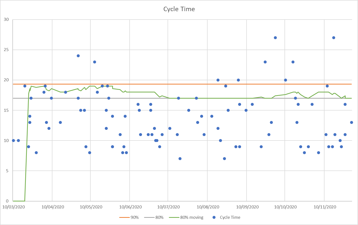
Convergence of the 80% percentile (green line). This line is plotted while the data is accumulated (the others take the data as historic data).
When we want to forecast more than one item we can make use of Monte Carlo simulations - but that is too large a topic to be squeezed in here. I will cover it with yet another blog post to come - hopefully soon.
Metrics for quality
In my recent blog post about business agility I have discussed that we need to complement efficiency of delivery with a focus on the creation of business value. I was also arguing in that article that the outcomes we expect from features and products are assumptions that need to be validated using the scientific method including the forming of a hypothesis and testing it.
However, there is one more aspect of reporting that is akin to business value: quality.
Similar to traditional efficiency metrics looking at progress tracking, quality is often reported on by bug counts, bug to fix ratios and trends for bugs or similar types of measures.
Working on a maturity assessment I have had a look at the organisations PMO reports and found all of those bug counting metrics. Asking the PMO representative if 124 bugs in the system means the quality was low the answer was an unsure facial expression. After a little thinking, they said the trend was sharply upwards so definitely negative.
Unfortunately, the context of the rise was that integration testing had just started and many already existing bugs were found. This does not mean the quality of the system deteriorated sharply, it only meant they didn’t know about them before. Also, 124 bugs in a very large and complex system is not necessarily bad. There was no accounting for severity, no note on how many bugs were accepted and put to the back-burner, no risk or impact stated. For me, this number was meaningless and certainly not an actionable metric as it does not convey enough information to decide on any action - not even that we should fix the bugs as they might all be minor and accepted to stay for now.
While discussing this problem of reporting on quality with my fantastic colleague from the test practice Elizabeth Fiennes I had the idea of using a different kind of approach to judging and reporting on quality: What if we focus on the practices currently used to achieve quality and add those outcome-based metrics like customer satisfaction that indicate quality?
This is what I have done in the below chart that resembles a heatmap with red, amber and green indication for each metric. The individual metrics are indicative only and not a specific recommendation.
What I like about the chart is that it highlights problem areas immediately and the metrics are actionable.
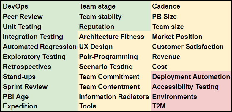
Red-Amber-Green chart showing practices influencing quality and outcome-based metrics supporting the notion of good or bad quality. Red: the practice is not used, amber: used but could do better, green: used as expected (we can always get better of course). Similar interpretation for the outcome-based metrics.
The basic idea is that each practice either has the potential to improve quality if done right, e.g. pair programming or indicates a judgement of the product that includes quality, e.g. customer satisfaction but also team contentment.
We colour a practice green if it is used correctly and to the expected extent. Amber if that is not the case but the practice is at least used to a basic level and red if it is not used at all or not correctly. This judgement is, of course, subjective and to avoid bias we want to make sure we have the right checks and balances in place. The same is true for the judgements, e.g. customer satisfaction or revenue.
However, we have this situation with any metric and its interpretation. What we need to do is to ask the right questions and trust that the people we are working with are doing their best, are not gaming if we don’t force them to by making a metric their target and are not acting out of maliciousness. To avoid gaming the key is for the people to feel safe to report reality, knowing they are not going to be blamed and that instead there is support available for them to fix issues.
Summary
We have covered the crucial metrics involved in Flow, explained how they help us with creating a predictable system, introduced Cumulative Flow Diagrams as a visual tool for investigating the state of our system and discussed how cycle time scatterplots can help us with forecasting single items.
If we want to create an efficient delivery capability Flow will give us the fundamentals and enable empiricism by enabling fast Build-Measure-Learn cycles.
As another metrics topic, we have also covered the idea to measure quality by practices used and outcome-based metrics that support a judgement of quality. A simple heatmap style chart provides an actionable set of metrics highlighting areas for improvement at a glance.
I am also promising another post on forecasting sets of work items, e.g. a Sprint, an Epic or all the work items representing a larger feature or theme, using Monte Carlo simulation - soon.
-
The original form of Little’s Law is $L=\lambda W$, with L = average number of customers, $\lambda$ = average arrival rate, W = average time a customer spends in the system. This form focuses on the arrival rate, the form used in my post is modified (not by myself) for looking at the departure rate instead ($\overline{TP}$ is describing the departure rate). The difference affects not only how the equation looks like but the assumptions themselves are different. If you are interested in more detail you can have a look at Daniel Vacanti’s book Actionable Agile Metrics for Predictability. ↩
-
There is an argument to have about how pairing exactly affects the amount of time needed to finish an item, follow-on effects due to increased quality and the difference between pairing on simple straightforward items vs complex items that need a lot of creativity. However, even if there is only a small amount of speed-up, the team will work on less items at any given time. Throughput could decrease but from experience, the gain in work in progress is larger than the slow-down. Many of the follow-on effects are not directly visible in Flow but can be looked at by monitoring technical debt and quality. For those interested have a look at this paper from Hannay et al. and this one from Alistair Cockburn and Laurie Williams and something more practical on Martin Fowler site. ↩