In my last article (on line annotation components for D3 charts), I created a component which calculated and displayed a moving average. As promised, I’m now turning my attention to Bollinger Bands.

Quick update - the code in this article was used as the starting point for components in the d3fc project. It’s a bit more advanced than this article, but you might find it interesting to see what this code evolved into!

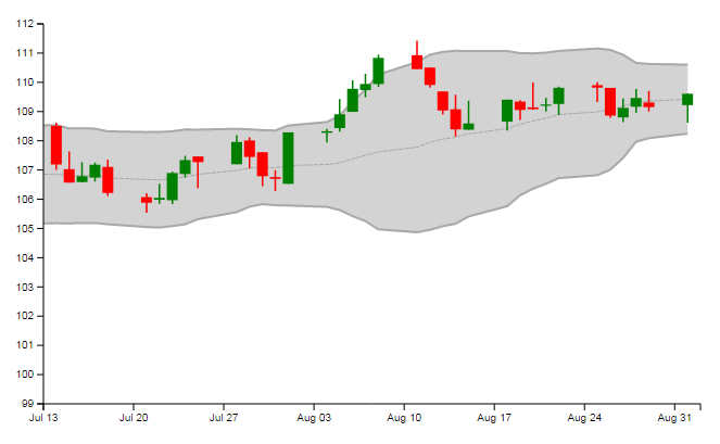
The component I’m going to create is going to look like this:

As before, I’m going to cheat by taking the chart Tom’s developed in his article on OHLC and candlestick components, and I’m creating the component following Mike Bostock’s convention.

What are Bollinger Bands?

Glad you asked. In a nutshell, Bollinger Bands are used on financial charts to indicate price volatility. As you can see from the chart above, they consist of three components:

• A moving average
• An upper band
• A lower band

The upper and lower bands are some number of standard deviations away from the moving average - and note that here we’re talking about a moving standard deviation. From this definition we can see that we need two parameters for our calculations - the moving average period, for which a value of 20 is typically used, and the number of standard deviations, which is typically 2.

Bollinger Bands Component

Here’s the complete code for the Bollinger Bands component - I’ll go through it below and explain what’s going on.

sl.series.bollinger = function () {

    var xScale = d3.time.scale(),
        yScale = d3.scale.linear();

    var yValue = 0,
        movingAverage = 20,
        standardDeviations = 2;

    var cssBandArea = 'bollingerBandArea',
        cssBandUpper = 'bollingerBandUpper',
        cssBandLower = 'bollingerBandLower',
        cssAverage = 'bollingerAverage';

    var bollinger = function (selection) {

        var areaBands = d3.svg.area(),
            lineUpper = d3.svg.line(),
            lineLower = d3.svg.line(),
            lineAverage = d3.svg.line();

        areaBands.x(function (d) { return xScale(d.date); });
        lineUpper.x(function (d) { return xScale(d.date); });
        lineLower.x(function (d) { return xScale(d.date); });
        lineAverage.x(function (d) { return xScale(d.date); });

        var calculateMovingAverage = function (data, i) {

            if (movingAverage === 0) {
                return data[i][yValue];
            }

            var count = Math.min(movingAverage, i + 1),
                first = i + 1 - count;

            var sum = 0;
            for (var index = first; index <= i; ++index) {
                var x = data[index][yValue];
                sum += x;
            }

            return sum / count;
        };

        var calculateMovingStandardDeviation = function (data, i, avg) {

            if (movingAverage === 0) {
                return 0;
            }

            var count = Math.min(movingAverage, i + 1),
                first = i + 1 - count;

            var sum = 0;
            for (var index = first; index <= i; ++index) {
                var x = data[index][yValue];
                var dx = x - avg;
                sum += (dx * dx);
            }

            var variance = sum / count;
            return Math.sqrt(variance);
        };

        selection.each(function (data) {

            var bollingerData = {};
            for (var index = 0; index < data.length; ++index) {

                var date = data[index].date;

                var avg = calculateMovingAverage(data, index);
                var sd = calculateMovingStandardDeviation(data, index, avg);

                bollingerData[date] = {avg: avg, sd: sd};
            }

            areaBands.y0(function (d) {

                var avg = bollingerData[d.date].avg;
                var sd = bollingerData[d.date].sd;

                return yScale(avg + (sd * standardDeviations));
            });

            areaBands.y1(function (d) {

                var avg = bollingerData[d.date].avg;
                var sd = bollingerData[d.date].sd;

                return yScale(avg - (sd * standardDeviations));
            });

            lineUpper.y(function (d) {

                var avg = bollingerData[d.date].avg;
                var sd = bollingerData[d.date].sd;

                return yScale(avg + (sd * standardDeviations));
            });

            lineLower.y(function (d) {

                var avg = bollingerData[d.date].avg;
                var sd = bollingerData[d.date].sd;

                return yScale(avg - (sd * standardDeviations));
            });

            lineAverage.y(function (d) {

                var avg = bollingerData[d.date].avg;

                return yScale(avg);
            });

            var prunedData = [];
            for (var index = movingAverage; index < data.length; ++index) {
                prunedData.push(data[index]);
            }

            var pathArea = d3.select(this).selectAll('.area')
                .data([prunedData]);
            var pathUpper = d3.select(this).selectAll('.upper')
                .data([prunedData]);
            var pathLower = d3.select(this).selectAll('.lower')
                .data([prunedData]);
            var pathAverage = d3.select(this).selectAll('.average')
                .data([prunedData]);

            pathArea.enter().append('path');
            pathUpper.enter().append('path');
            pathLower.enter().append('path');
            pathAverage.enter().append('path');

            pathArea.attr('d', areaBands)
                .classed('area', true)
                .classed(cssBandArea, true);
            pathUpper.attr('d', lineUpper)
                .classed('upper', true)
                .classed(cssBandUpper, true);
            pathLower.attr('d', lineLower)
                .classed('lower', true)
                .classed(cssBandLower, true);
            pathAverage.attr('d', lineAverage)
                .classed('average', true)
                .classed(cssAverage, true);

            pathArea.exit().remove();
            pathUpper.exit().remove();
            pathLower.exit().remove();
            pathAverage.exit().remove();
        });
    };

    // NOTE: The various get / set accessors would go here
    // but I've removed them in the interest of readability

    return bollinger;
};

That’s a decent amount of code, so let’s start at the top by looking at the properties I’ve defined on this component - you’ll see that I’ve broken them down into sections so we don’t have a monolithic block of declarations at the top of the file.

• First we have the X and Y scales, which the component needs when it’s working out where to draw things.
• Next we have the fields we need to perform our calculations - the field to use on the data model, the moving average period, and the number of standard deviations to use. Note that we’re defaulting the moving average period to 20 and the number of standard deviations to 2, the typical values for these fields.
• Finally we have a number of properties which define CSS classes for the various parts of the component. This provides the user with a lot of customisability when it comes to styling, but we set default values so that the user doesn’t have to specify these properties.

In the component function we create a d3.svg.area to represent the area between the upper and lower bands, and three d3.svg.line objects to represent the upper band, lower band, and moving average line, setting their X-values appropriately. I’m using the area element because that’s a really nice, built-in way to show the area between two lines. The best part is, it’s really simple to use - where a line element requires you to set its Y-value, an area element has two Y-values - and I’m very much in favour of making life easy for myself.

In the next section we define two functions to calculate the moving average and the moving standard deviation. Note that Bollinger Bands use the population version of the standard deviation formula.

Inside the selection.each block is where we do our heavy lifting - setting the Y-values of our various SVG elements. We declare an empty variable, bollingerData, then we populate it with data - it’s a map of date to avg (moving average) and sd (standard deviation) for each data item. We do this once, which is massively more efficient than it would be if we did all these calculations on the fly! On the other hand, this means we’re doing these calculations every time the component is redrawn; if we wanted to be maximally efficient we’d cache this information, but that would also require us to check that the data hadn’t changed every time we needed to redraw, which brings its own problems. The remainder of the selection.each block is lengthy but pretty simple - we’re just setting the Y-values for our area and line elements based on the data in the bollingerData map.

Finally we add the areaBands, lineUpper, lineLower and lineAverage SVG elements to the path. Note that we don’t set the whole of the data array on these elements - Bollinger Bands typically aren’t shown when there’s not enough data to calculate the full moving average, so we start at index movingAverage, which has the desired effect.

I’ve not shown the various get/set accessors because they’re not especially interesting, as they’re pretty much all the same:

bollinger.yValue = function (value) {
    if (!arguments.length) {
        return yValue;
    }
    yValue = value;
    return bollinger;
};

Adding the component to the chart

OK, that’s the tricky bit out of the way, so now let’s use this new Bollinger Bands component.

First we create and configure our component:

var bollinger = sl.series.bollinger()
    .xScale(xScale)
    .yScale(yScale)
    .yValue('close')
    .movingAverage(20)
    .standardDeviations(2);

Here we’re just telling the component about the X and Y scales, and telling it to use the ‘close’ property on the data model. The movingAverage and standardDeviations properties are optional (especially since we’re just setting them to their default values here, but you’d need to include them if you wanted anything non-standard). We could also set any of the four CSS properties that the component exposes, but I’ve chosen to omit them here and just leave them with their default values.

With that done, we add the component to the chart:

plotArea.append('g')
    .attr('class', 'bollinger')
    .datum(data)
    .call(bollinger);

Pro tip: I’m putting this code just in front of the code to display the chart data itself, so that the Bollinger Bands will be in the background and the chart data will be in the foreground.

Styling

Obviously, the last step is to style the various sections of the component.

.chart .bollingerBandArea {
    fill: lightgrey;
    stroke-width: 0;
}

.chart .bollingerBandUpper {
    fill: none;
    stroke: darkgrey;
    stroke-width: 2;
}

.chart .bollingerBandLower {
    fill: none;
    stroke: darkgrey;
    stroke-width: 2;
}

.chart .bollingerAverage {
    fill: none;
    stroke: darkgrey;
    stroke-width: 1;
    stroke-dasharray: 4, 1;
}

I’ve chosen to display the Bollinger Bands in grey, so I’m using a light grey for the area between the upper and lower bands and a darker grey for the bands themselves (you could instead use transparency to make the area lighter).

As an aside, note that I’ve set stroke-width: 0 on the area so that it doesn’t show any borders. I’ve done this for two reasons. firstly, we’re drawing over the top and bottom borders anyway, and secondly we don’t want a left or right border to be shown - try removing this line and you’ll see what I mean.

Putting it all together, this is the result:

Enhancements

I’m pretty happy with this component - it works really well and it’s reasonably efficient, programmatically. There are still a few enhancements we could do though. If you read through the Wikipedia entry on Bollinger Bands you’ll see that we’re using a simple moving average calculation, but that other types of calculation are sometimes used; we could extend our component to allow the user to choose by providing an additional property like .movingAverageType('exponential').

Conclusion

In this article I’ve taken the moving average component I developed in my previous article and used it as the basis for a Bollinger Bands component. The new component is very easy to configure and style.