Financial traders who make their living (or at least some extra spending money) from the financial markets have developed a whole host of indicators that overlay the price of an instrument, providing signals for when to buy or sell.

As well as indicators, traders also make use of some quite specialised, non time-series, chart types. Market profile charts are one such example. In brief, a market profile chart groups prices together into discrete time-periods. For each time-period a histogram is presented that shows the volume traded at each price interval. As a result, the longest horizontal bar is the price where most volume has been traded.

Here’s an example chart:

You can find out how to read (and trade from) a market profile on various websites. In this post I’m more concerned with how to render this unusual looking chart!

Creating a market profile histogram

To render the market profile chart I’m going to be using a combination of D3 and d3fc (which provides a number of components that complement and extend D3).

The first step is to obtain some suitable data. Rather than hunt around for price data in CSV / JSON format, I’m going to use one of the d3fc random data generators:

const timePeriods = 40;

const generator = fc.randomFinancial()
  .interval(d3.timeMinute)
const timeSeries = generator(timeUnits);

This generates a time series of 40 points, at one minute intervals, using a geometrical brownian motion generator, which gives quite realistic looking data.

[
  {
    date: 2016-01-01T00:00:00.000Z,
    open: 100,
    high: 100.37497903455065,
    low: 99.9344064016257,
    close: 100.13532170178823,
    volume: 974
  },
  {
    date: 2016-01-01T00:01:00.000Z,
    open: 100.2078374019404,
    high: 100.55251268471399,
    low: 99.7272105851512,
    close: 99.7272105851512,
    volume: 992
  },
  ...
]

In order to create the market profile histogram, a suitable set of price ‘buckets’ needs to be calculated. The d3 scale ticks function is a convenient method for creating these buckets, providing values that are “uniformly spaced, have human-readable values, and are guaranteed to be within the extent of the domain”.

The following code computes the extent of the prices within this time series using the d3fc extent component, then uses a d3 linear scale to create the buckets:

// determine the price range
const extent = fc.extentLinear()
  .accessors([d => d.high, d => d.low]);
const priceRange = extent(timeSeries);

// use a d3 scale to create a set of price buckets
const priceScale = d3.scaleLinear()
  .domain(priceRange);
const priceBuckets = priceScale.ticks(20);

This produces an array of buckets as follows:

[99.96, 99.965, 99.97, ..., 100.035, 100.04]

The construction of the profile itself is probably easiest to understand visually. The first step is to overlay the time series with a set of boxes where trading occurred within each time period:

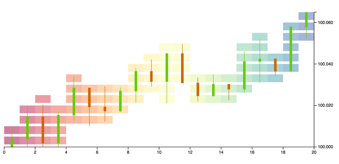
This is called a ‘split profile’ chart. To form a market profile, you weight each box based on the volume for that time period, then ‘slide’ them to the left in order to stack them up.

Here’s a function that calculates the market profile chart for a time series:

const createMarketProfile = (data, priceBuckets) => {
  // find the price bucket size
  const priceStep = priceBuckets[1] - priceBuckets[0];

  // determine whether a datapoint is within a bucket
  const inBucket = (datum, priceBucket) =>
    datum.low < priceBucket && datum.high > (priceBucket - priceStep);

  // the volume contribution for this bucket
  const volumeInBucket = (datum, priceBucket) =>
    inBucket(datum, priceBucket)
      ? datum.volume / Math.ceil((datum.high - datum.low) / priceStep) : 0;

  // map each point in our time series, to construct the market profile
  const marketProfile = data.map(
    (datum, index) => priceBuckets.map(priceBucket => {
      // determine how many points to the left are also within
      // this time bucket
      const base = d3.sum(data.slice(0, index)
                    .map(d => volumeInBucket(d, priceBucket)));
      return {
        base,
        value: base + volumeInBucket(datum, priceBucket),
        price: priceBucket
      };
    })
  );

  // similar to d3-stack - cache the underlying data
  marketProfile.data = data;
  return marketProfile;
};

The output of the above function is similar to the output of d3.stack.

Rendering a stacked bar chart is pretty straightforward using a couple of d3fc series components. A bar series component is used to render the data for each time period, with a repeat series creating a bar for each of the periods.

The repeat series is ‘decorated’ in order to assign a fill colour for each series based on its index:

const colorScale = d3.scaleSequential(d3.interpolateSpectral)
  .domain([0, timePeriods]);

const barSeries = fc.autoBandwidth(fc.seriesSvgBar())
    .orient('horizontal')
    .align('left')
    .crossValue(d => d.price)
    .mainValue(d => d.value)
    .baseValue(d => d.base);

const repeat = fc.seriesSvgRepeat()
  .series(barSeries)
  .orient('horizontal')
  .decorate((selection) => {
    selection.enter()
      .each((data, index, group) =>
        d3.select(group[index])
          .selectAll('g.bar')
          .attr('fill', () => colorScale(index))
      );
  });

This series is rendered via a d3fc cartesian chart.

const chart = fc.chartSvgCartesian(
    d3.scaleLinear(),
    d3.scaleBand()
  )
  .xDomain(xExtent(_.flattenDeep(marketProfile)))
  .yDomain(priceBuckets)
  .yTickValues(priceBuckets.filter((d, i) => i % 4 == 0))
  .plotArea(repeat);

d3.select('#chart')
  .datum(marketProfile)
  .call(chart);

This produces a complete market profile for this time period:

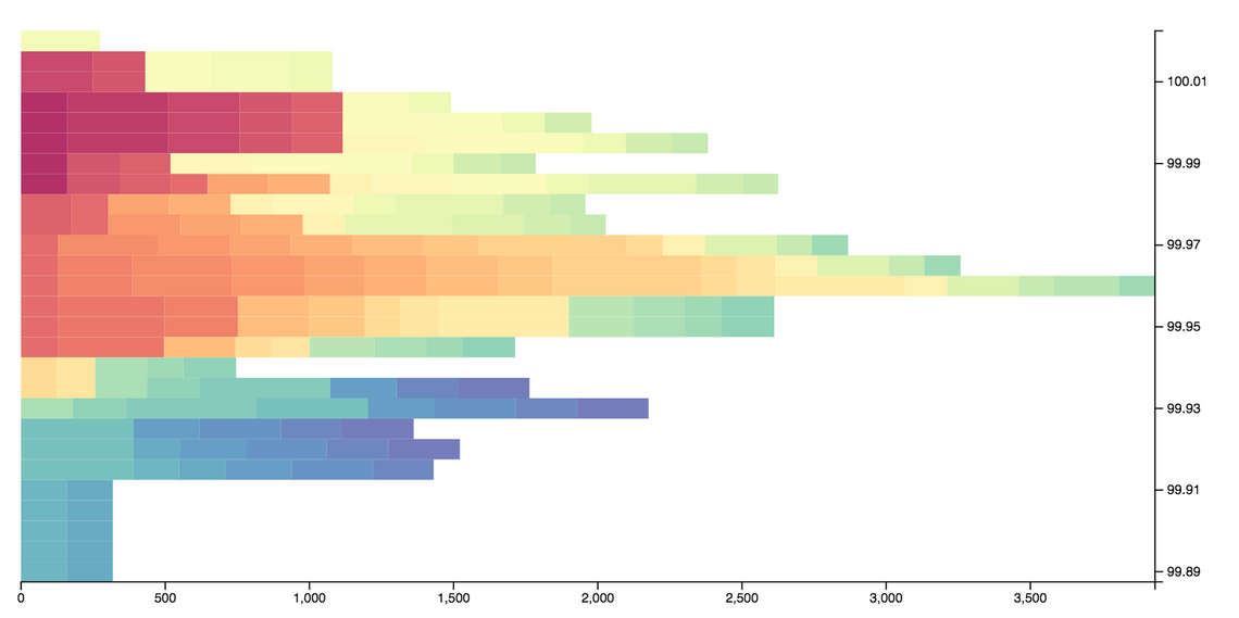
The complete code for this example is on the bl.ocks website.

Rendering multiple profiles

The chart above provides the profile for a single time period. Typically market profile charts show the price/volume histogram for multiple time periods, a much more challenging charting problem!

Using the createMarketProfile function above it is quite easy to create a number of profiles for a single time series:

const series = _.chunk(timeSeries, 12)
  .map((data) => createMarketProfile(data, priceBuckets));

The above code uses the lodash chunk function to split the array into ‘chunks’ each containing 12 ‘candlesticks’. This is mapped via the createMarketProfile function to provide the profile for each of these chunks.

When rendering the profiles for multiple time periods the x-scale is no longer a straightforward linear scale, instead each of the time periods has its own scale. A good way to approach this problem is to use an ordinal x scale to provide the overall chart layout, then use a ‘nested’ linear scale for each profile.

The d3 band scale creates discrete sub-divisions, with padding, where the bandwidth function returns the computed bandwidth based on the scale’s domain and range:

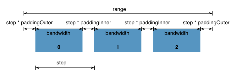
(Image from the d3 band scale documentation)

With d3fc, the bandwidth value returned by the scale is propagated to the series, via the autobandwidth component.

An easy way to make use of the bandwidth provided by the x-scale, and construct a nested linear scale for each profile, is to construct a new series component. Here’s the basic scaffolding:

const seriesMarketProfile = () => {
  let xScale, yScale, bandwidth;

  const barSeries = // ...;
  const colorScale = // ...;
  const repeatSeries = // ...;

  const series = (selection) => {
    selection.each((data, index, group) => {

      // rendering logic goes here ...
    })
  };

  // standard d3 property accessors
  series.xScale = (...args) => { };
  series.bandwidth = (...args) => { };
  series.yScale = (...args) => { };

  return series;
}

The series has xScale and yScale properties, which are common properties of all d3fc series, and a bandwidth property which receives the bandwidth from the scale. The above code follows the d3 component pattern having property accessors and returning a function that receives a selection (so that it can be used via select.call). The barSeries, colorScale and repeatSeries are exactly the same as those in the single profile example.

Now for the clever part, the rendering logic! (which is actually quite simple)

For each datapoint (which is a price / volume profile), a linear scale is constructed, with a range computed from the series’ scale (or outer-scale). Other than that, the rendering logic is exactly the same as the simpler single profile version.

const series = (selection) => {
  selection.each((data, index, group) => {

    // compute the largest value across all of our profiles
    const xDomain = d3.extent(_.flattenDeep(data).map(d => d.value));

    colorScale.domain([0, data.length]);

    join(d3.select(group[index]), data)
      .each((marketProfile, index, group) => {

        // create a composite scale that applies the required offset
        const leftEdge = xScale(marketProfile.data[0].date);
        const offsetScale = d3.scaleLinear()
            .domain(xDomain)
            .range([leftEdge, leftEdge + bandwidth]);

        repeatSeries.yScale(yScale)
            .xScale(offsetScale);

        // render
        d3.select(group[index])
          .call(repeatSeries);
      });
  })
};

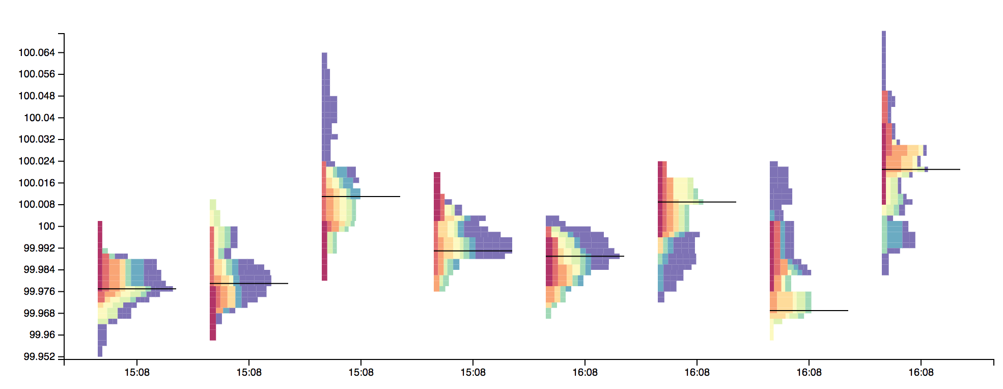
Market profile charts also have various other annotations, such as the Point Of Control (POC), which is the price with maximum volume for each time period. I’ve added the POC by adapting an error bar series, I’ll not go into the details here, if you’re interested, take a look at the code.

Here’s the final chart:

The complete code for this example is on the bl.ocks website.

I certainly had fun putting this example together, a pretty complex chart that provides a good illustration of d3 and the d3fc components.