Only a month ago I walked through a simple application of Machine Learning (ML) with Scikit Learn. This library offers an abundance of ML tools for data classification, which I hope I showed to be a relatively painless task. However, I’d experimented with Scikit Learn before, and thought, where’s the fun in that? It’s time to dive into a new library which has also attracted a big name for itself: TensorFlow.

Adopted by Coca Cola, Google, and Twitter, to name a few, TensorFlow has found itself to be the most loved library by respondents to the Stack Overflow 2018 Developer Survey. TensorFlow was the work of the Google Brain Team before becoming open-source. I’ll walk through a simple application of TensorFlow, using the same dataset as Scikit Learn and the latest version of Python 3 (v3.6.4 at the time of writing). If you haven’t yet found a chance to read my article demonstrating Scikit Learn, I would strongly advise reading the setup for a better understanding of the dataset we’re going to use.

Installation

Before installing TensorFlow, first make sure to download and install a 64-bit version of Python 3. Whilst Scikit Learn executed happily with a 32-bit version, the same does not apply to TensorFlow. With your terminal open, TensorFlow is installed in a single pip command:

pip install tensorflow

In order to read CSV files for this walkthrough, we’ll also require Pandas as before:

pip install pandas

That’s us ready to go!

Setup

Given that the details about the dataset from UCI are discussed in detail in the setup for Scikit Learn, I’ll keep this one concise. Exactly as before, we use Pandas to import two CSV files which contain image samples of handwritten digits:

import pandas as pd

def retrieveData():
  trainingData = pd.read_csv("training-data.csv", header=None).as_matrix()
  testData = pd.read_csv("test-data.csv", header=None).as_matrix()

  return trainingData, testData

Each row in our training and test datasets contains one sample, formed from one feature vector of length 16 followed by one corresponding category. The feature vector describes the image by sampling the intensity of 16 pixels, whilst the category explicitly states which digit has been written in the image. Similar to before, we’ll split categories from their feature vectors for convenience:

def separateFeaturesAndCategories(trainingData, testData):
    trainingFeatures = formatFeatures(trainingData[:, :-1])
    trainingCategories = trainingData[:, -1:]
    testFeatures = formatFeatures(testData[:, :-1])
    testCategories = testData[:, -1:]

    return trainingFeatures, trainingCategories, testFeatures, testCategories

One difference exists here from our Scikit Learn example: The application of formatFeatures to both training features and test features in our datasets. TensorFlow takes these features in the form of a Python dictionary, as opposed to an array like Scikit Learn. Given that each feature vector represents 16 pixels, our dictionary will contain 16 key-value pairs: The keys corresponding to pixels, and values corresponding to their intensities. In other words, key i of our dictionary corresponds to pixel i from each sample in our dataset:

def formatFeatures(features):
    formattedFeatures = dict()
    numColumns = features.shape[1]

    for i in range(0, numColumns):
        formattedFeatures[str(i)] = features[:, i]

    return formattedFeatures

Instantiating the Classifier

Before we proceed to instantiate a classifier tool (the “classifier”), TensorFlow requires further information about the type of data its classifier is expected to handle. This is articulated through TensorFlow’s feature column object. Luckily for us, all our data is numeric, so our feature columns need not be particularly sophisticated. By iterating over our feature dictionary keys we can create a feature column for each and specify the numeric type by introducing a numeric_column:

import tensorflow as tf

def defineFeatureColumns(features):
    featureColumns = []

    for key in features.keys():
        featureColumns.append(tf.feature_column.numeric_column(key=key))

    return featureColumns

With feature columns ready for use, instantiating a classifier is a relatively painless task, much like Scikit Learn! Instead of working with a Stochastic Gradient Descent (SGD) classifier like before, we’ll take advantage of Tensorflow’s DNN classifier. Before proceeding to show you the implementation, it would be beneficial to describe the general structure of the DNN.

DNN stands for Deep Neural Network. This type of network is designed to function like a human brain, consisting of multiple layers of nodes. These nodes act like neurons in the brain, where the computation takes place. Every DNN consists of one input layer, one output layer, and multiple “hidden” layers. The number of hidden layers is configurable, and differs from DNN to DNN. These networks recognise patterns in numeric data as the data is filtered between layers, starting with the input layer and finishing in the output layer.

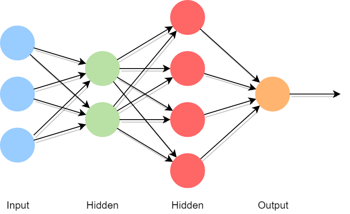
With the general structure in mind, we proceed to instantiate a TensorFlow DNN with three parameters:

1. feature_columns, the array of feature column objects we defined earlier
2. hidden_units, a list indicating the number of nodes for each hidden layer
3. n_classes, an integer > 1 which indicates the number of categories in our data

Notice that the majority of information for the structure of the network is inferred from hidden_units. The length of the list dictates the number of hidden layers our network contains, and each value within the list establishes the number of nodes in these layers. The implementation itself boils down to a few lines of code:

def instantiateClassifier(featureColumns):
    classifier = tf.estimator.DNNClassifier(
        feature_columns = featureColumns,
        hidden_units = [20, 30, 20],
        n_classes = 10
    )

    return classifier

Training

With a DNN instantiated, it’s time to provide training. There are two questions to consider at this stage: What should we do if our DNN is working with an exceptionally large set of data, and how often should the DNN iterate over the data before it’s sufficiently trained? The first question is relatively simple to answer: Break down the data into smaller batches, and feed data to the DNN one batch at a time. Our DNN will be training with ~7500 samples, so let’s break this down into batches of 100 samples.

The second question, on the other hand, is trickier to answer. Try a range of numbers, and see what delivers the best results for you! Keep in mind, too few iterations may mean the DNN has missed some important trends in your data, whilst too many iterations may mean the DNN concentrates too much on less significant trends! Pinpointing the optimal number of iterations is a difficult task. For the sake of demonstrating how this works, let’s set our DNN to run 50 iterations, or “steps”.

def train(features, labels, batchSize):
    dataset = tf.data.Dataset.from_tensor_slices((dict(features), labels))

    return dataset.shuffle(1000).repeat().batch(batchSize)

def trainClassifier(classifier, trainingFeatures, trainingCategories):
    classifier.train(
        input_fn = lambda:train(trainingFeatures, trainingCategories, 100),
        steps = 50
    )

Observe that TensorFlow calls train for each step of the training. This function formats the data as a TensorFlow dataset, and proceeds to train the classifier data for each batch of 100 samples. Once its done, the TensorFlow dataset will be reshuffled, and the training resumes. This is repeated 1000 times, completing a single step of the training. We’re left to repeat this whole process 50 times. This sounds like an exceptional amount of work! Once all 50 steps are complete, our classifier is ready for testing.

Evaluation

We’ll base the success of this classifier on its accuracy score, which is determined by comparing the classifier’s predictions to the categories from our test dataset, and taking the fraction of predictions which match the given categories. We apply similar code to what we observed at the training stage, replacing the training data with the test data and omitting the steps argument:

def test(features, labels, batchSize):
    dataset = tf.data.Dataset.from_tensor_slices((dict(features), labels)).batch(batchSize)

    return dataset

def testClassifier(classifier, testFeatures, testCategories):
    accuracy = classifier.evaluate(
        input_fn = lambda:test(testFeatures, testCategories, 100)
    )

    return accuracy

And there we have it! A fully trained and tested TensorFlow Deep Neural Network classifier. That’s a mouthful! Two questions spring to mind now which fill my curiosity:

1. How well does the DNN perform?
2. How does this compare to Scikit Learn’s SGD classifier?

To answer the first question, running our DNN several times has given a particularly impressive average score of 78%! This doesn’t quite match up to the bar set by Scikit Learn - sitting on 84% - but there are plenty of parameters to play with which may well allow the DNN to beat this record. As I discussed in my previous article, there’s an abundance of parameters to experiment with, and plenty of potential to either improve or worsen our results: We could introduce more nodes to our hidden layers, add more hidden layers, or increase the number of steps in the training process.

One key point to make in comparing these two libraries is that Scikit Learn included a pre-processing stage to standardise the data we were working with. I haven’t done the same for TensorFlow, but implementing this step in the pipeline would require only a little extra work. Even without pre-processing, I think TensorFlow has done a grand job with the basic DNN setup here. Whilst I’ve only measured the accuracy score here, TensorFlow offer’s a module’s worth of metrics for further analysis of the results.

Conclusion

This brings to an end the second application of ML using Python! Before attempting to work with TensorFlow, I led myself to believe the setup would prove more challenging than Scikit Learn. However, this wasn’t at all the case. Formatting the features into Python dictionaries seemed a little tedious, since this wasn’t necessary in Scikit Learn, but the process of instantiating, training, and testing a TensorFlow classifier was relatively straightforward.

In the end, the results for each library with next-to-no experimentation of parameters were both excellent, and I would be happy to recommend either library to anyone considering the process of building a ML tool in the near future! If, like me, you’re keen to explore TensorFlow further, I find its well documented on their own website. Better still, if you’re keen to add improvements and extra features to the code seen here, you’re more than welcome to play with the DNN on GitHub. Happy coding!