You know my methods, Watson. There was not one of them which I did not apply to the inquiry. And it ended by my discovering traces, but very different ones from those which I had expected.

The Memoirs of Sherlock Holmes (1893)

Apache Spark is well known in the Big Data community for its incredible performance and expressive API. However, it just takes one small misstep to transform a massively parallel powerhouse into a pathetically poor performer. This post presents an example and the steps that can be taken to discover the root of the problem.

A simple DataFrame

Normally when working with Spark, not having enough data is the last of your problems. In fact, when it comes to prototyping operations, too much data can be a hindrance. It can be very handy to generate a smallish dataset to play with. So for our example, let’s start by creating a DataFrame of the numbers 0 to 1 million.

What could be simpler?

Suppose we created a User Defined Aggregation Function (UDAF) that does some complex number crunching. Now we can go ahead and test it out. But, hang on a minute, I didn’t expect it to take that long. Some quick back of the envelope calculations later … you find it would take days to process your data.

How to diagnose poor performance

Step 1: Isolate the problem

It is always good to test your Spark jobs incrementally: taking each piece individually and ensuring that the time to complete the job is in line with your expectations. A simple benchmarking function that executes the job a number of times is also helpful. So being the diligent developer, you’ve already narrowed down your problem to this one new piece of your pipeline. Great!

Step 2: Find long-running Tasks in the Spark UI timeline

The Spark UI is an endlessly helpful tool that every Spark developer should become familiar with. It can be confusing at first, so you need to have an understanding of how Spark splits work into Jobs then Stages then Tasks.

We have a Job that creates a DataFrame then performs an aggregation on that DataFrame. Aggregations are Wide Transformations so they form a new Stage. Each piece of work that sits within a Stage is a Narrow Transformation, like a map transformation. By running your Job on your local machine rather than a shared cluster you have full control over the jobs that will be executed, making it easier to find your job in the UI (it’s the only one!). The first thing I do is check the timeline of Jobs which should confirm that there is a problem.

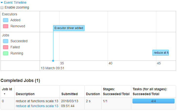
It took only 2 seconds, that’s not so terrible? But the average time was a lot longer when benchmarking… Something fishy is going on. Ok, let’s dig deeper, clicking on the job takes us to the Stage.

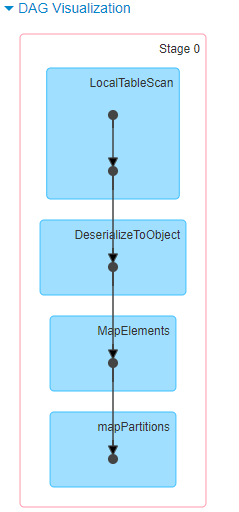
The DAG could hardly be more straightforward. As stated there is just one Wide transformation in our Job hence the linear pipeline of tasks. Let’s keep going, down to the Task granularity, and check the timeline.

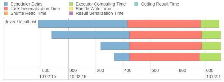
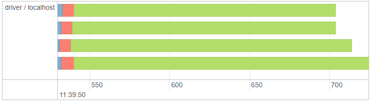
Now this is interesting. See all that red and blue? This is a sure sign that something is up. What we really want to see is lots of green - the proportion of time spent doing work - I mean real work - the part where Spark does the number crunching.

On this machine I have 4 cores, hence the 4 executors. Scheduler delay (blue) is the time spent waiting. There is something that the executors are waiting for - often this is waiting for the driver that controls and coordinates the jobs. Next we have a large chunk of red which is task deserialization time. The task is the set of instructions required to complete some work - essentially your code. This should not take up such a large proportion of time and it’s likely to be related to the scheduler delay.

Step 3: Compare with an equivalent

So we know that our task is taking a long time to deserialize, but why is that? At this point the cause is still not clear, so it can be helpful to contrast your job with an equivalent job that is known to be well performing.

Our job just consists of an aggregation (UDAF), so we can simply swap it for one of Spark’s aggregation functions and the DAG should look very similar. Next we check and contrast the results in the Spark UI.

In this case, the Job execution time is similar (in fact slightly longer). There are 2 Stages - one is for the collect which just takes the result of each executor, combines them, then sends back the result. Of the 2 stages. the longer running one is our equivalent. Let’s see its Task timeline.

No, you’re not seeing double. Yes, it looks just like the timeline from our UDAF. Alarm bells should be ringing. The Sherlocks among you may have already deducted the cause of the problem, for the rest of us, let’s take out one more tool from our detective’s handbook. We ask directly, “explain yourself!?”

Step 4: Explain

df.agg(mean("value")).explain

The result:

== Physical Plan ==
*(2) HashAggregate(keys=[], functions=[avg(cast(value#1 as bigint))])
+- Exchange SinglePartition
   +- *(1) HashAggregate(keys=[], functions=[partial_avg(cast(value#1 as bigint))])
      +- LocalTableScan [value#1]

This tells us the plan of the Job that Spark is going to execute. There is one thing that is odd about this. Why is there a LocalTableScan? We found the same issues in our Job with both our UDAF and with Spark’s aggregation mean. We know there is nothing wrong with Spark’s mean. Quoting Sir Arthur Conan Doyle:

When you have eliminated the impossible, whatever remains, however improbable, must be the truth.

Suppose there’s nothing wrong with our UDAF, then the problem must lie with the remaining code. Let’s see what explain gives us on our DataFrame with df.explain.

== Physical Plan ==
LocalTableScan [value#1]

Sure enough, creating our DataFrame is the part of the Plan that corresponds to the LocalTableScan above. Is there something wrong with the way we are generating our data? At this point, I’ll cut to the chase. Yes - we should be doing it like this:

And if we look at what explain tells us about this version of the DataFrame:

== Physical Plan ==
*(1) SerializeFromObject [input[0, int, false] AS value#2]
+- Scan ExternalRDDScan[obj#1]

We see that there are 2 steps. First there is some serialization going on, secondly there is a scan of an External RDD. Let’s take a quick look at the difference in performance.

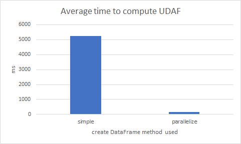
That’s a whopping 30x faster. (The average was computed from 10 iterations)

I know where you live

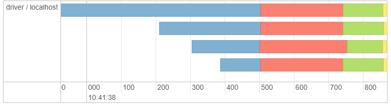
The reason our first DataFrame destroyed our performance is because of where it lives. It is often said how important it is to “know your data”, and I add to this: “know where your data is”. The poor performance was all because our data did not live where our executors could easily access it. Remember the large chunk of red Task Deserialization time - that was our entire DataFrame being serialized and sent to each Executor to process. In contrast, look at the timeline for our improved version:

Not only is the red deserialization a much healthier proportion of the whole task, it’s also a tiny fraction of time in comparison to before (8ms vs 240ms).

The way we created the DataFrame meant that it was living in-memory on the driver and not distributed across the cluster.

Conclusion

Although Spark is arguably the most expressive, flexible and powerful parallel processing engine around - it will only do exactly what you tell it to do. When your code doesn’t work as expected, it can be much harder to find the root cause than with a typical application bug.

I hope the tips highlighted here can serve others in easing that process. Of course, every issue is unique and may merit a bespoke approach at diagnosis. While a deep understanding of how clustered computing works in general is a must have, knowing your way around the Spark UI can quickly lead you in the right direction.