As a bit of a thought experiment, I wondered how hard it would be to create a cubic spline interpolation within Alteryx. As with many of my experiments BaseA rules apply.

Stealing an idea from Tasha Alfano, I thought I would do it in both Python and Alteryx from first principles. A quick shout out to MathAPI - a handy site and used to render all the LaTeX to SVG.

So let’s start by reviewing how to create a cubic spline and then build it up. I chose to use the algorithm as described in Wikiversity. Specifically with type II simple boundary conditions. I’m not going through the maths but will define the steps to build the spline.

Building a Tridiagonal Matrix and Vector

First, step is given an X array and a Y array of equal length n (greater than 2), we want to build a tridiagonal matrix which we will then solve to produce the coefficients for the piece-wise spline. The goal of the spline is that it hits every point (x, y) and that the first and second derivatives match at these points too.

Sticking with notation in the paper, lets define H to be an n-1 length array of the differences in X:

for

A tridiagonal matrix is a square matrix where all values except for the main diagonal and first diagonals below and above this. For example:

1   2   0   0
2   3   2   0
0   2   3   2
0   0   2   1

One advantage of a tridiagonal matrix is that they are fairly straight forward to invert and solve linear equations based on them. For the sake of coding up the algorithm - let’s define B to be the n length array holding the diagonal elements, A to be the n-1 length array of the diagonal above this and C to be the n-1 length array of the diagonal below:

b0   c0    0    0
a0   b1   c1    0
 0   a1   b2   c2
 0    0   a2   b3

Please note the indexes here are different from those used in the Wikiversity article, as they align with a standard array starting at 0. For the spline, these are arrays are given by:

for

for

for

Using the simple boundary condition that the second derivative is equal to 0 at the end, gives the values for c₀ and a_n-2 both equal to 0. This can easily be coded up in Python:

from typing import Tuple, List

def compute_changes(x: List[float]) -> List[float]:
    return [x[i+1] - x[i] for i in range(len(x) - 1)]

def create_tridiagonalmatrix(n: int, h: List[float]) -> Tuple[List[float], List[float], List[float]]:
    A = [h[i] / (h[i] + h[i + 1]) for i in range(n - 2)] + [0]
    B = [2] * n
    C = [0] + [h[i + 1] / (h[i] + h[i + 1]) for i in range(n - 2)]
    return A, B, C

The next step is to compute the right-hand side of the equation. This will be an array of length n. For notation, let’s call this D - the same as in the Wikiversity article:

for

Implementing this in Python looks like:

def create_target(n: int, h: List[float], y: List[float]):
    return [0] + [6 * ((y[i + 1] - y[i]) / h[i] - (y[i] - y[i - 1]) / h[i - 1]) / (h[i] + h[i-1]) for i in range(1, n - 1)] + [0]

Solving the Tridiagonal Equation

To solve a tridiagonal system, you can use Thomas Algorithm. Mapping this onto the terminology above. We first derive length n vectors C’ and D’:

for

for

Having worked out C’ and D’, calculate the result vector X:

for

The implementation of this in Python is shown below:

def solve_tridiagonalsystem(A: List[float], B: List[float], C: List[float], D: List[float]):
    c_p = C + [0]
    d_p = [0] * len(B)
    X = [0] * len(B)

    c_p[0] = C[0] / B[0]
    d_p[0] = D[0] / B[0]
    for i in range(1, len(B)):
        c_p[i] = c_p[i] / (B[i] - c_p[i - 1] * A[i - 1])
        d_p[i] = (D[i] - d_p[i - 1] * A[i - 1]) / (B[i] - c_p[i - 1] * A[i - 1])

    X[-1] = d_p[-1]
    for i in range(len(B) - 2, -1, -1):
        X[i] = d_p[i] - c_p[i] * X[i + 1]

    return X

Calculating the Coefficients

So the last step is to convert this into a set of cubic curves. To find the value of the spline at the point x, you want to find j such that x_j < x < x_j+1. Let’s define z as

z has property of being 0 when x = x_j and 1 when x = x_j+1. The value of spline at x, S(x) is:

Now to put it all together and create a function to build the spline coefficients. The final part needed is to create a closure and wrap it up as a function which will find j and then evaluate the spline. There is an excellent library in Python, bisect which will do a binary search to find j easily and quickly.

The code below implements this, and also validates the input arrays:

def compute_spline(x: List[float], y: List[float]):
    n = len(x)
    if n < 3:
        raise ValueError('Too short an array')
    if n != len(y):
        raise ValueError('Array lengths are different')

    h = compute_changes(x)
    if any(v < 0 for v in h):
        raise ValueError('X must be strictly increasing')

    A, B, C = create_tridiagonalmatrix(n, h)
    D = create_target(n, h, y)

    M = solve_tridiagonalsystem(A, B, C, D)

    coefficients = [[(M[i+1]-M[i])*h[i]*h[i]/6, M[i]*h[i]*h[i]/2, (y[i+1] - y[i] - (M[i+1]+2*M[i])*h[i]*h[i]/6), y[i]] for i in range(n-1)]

    def spline(val):
        idx = min(bisect.bisect(x, val)-1, n-2)
        z = (val - x[idx]) / h[idx]
        C = coefficients[idx]
        return (((C[0] * z) + C[1]) * z + C[2]) * z + C[3]

    return spline

The complete python code is available as a gist:

Testing the Spline

As always, it is essential to test to make sure all is working:

import matplotlib.pyplot as plt

test_x = [0,1,2,3]
test_y = [0,0.5,2,1.5]
spline = compute_spline(test_x, test_y)

for i, x in enumerate(test_x):
    assert abs(test_y[i] - spline(x)) < 1e-8, f'Error at {x}, {test_y[i]}'

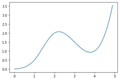
x_vals = [v / 10 for v in range(0, 50, 1)]
y_vals = [spline(y) for y in x_vals]

plt.plot(x_vals, y_vals)

Creates a small spline and ensure that the fitted y values match at the input points. Finally, it plots the results:

Recreating In Alteryx

So that’s the full process, now to rebuild it in Alteryx using BaseA. For the input, the macro takes two separate inputs - a table of KnownXs and KnownYs and a list of target Xs. Again, the first task is to build H, A, B, C, D from the inputs:

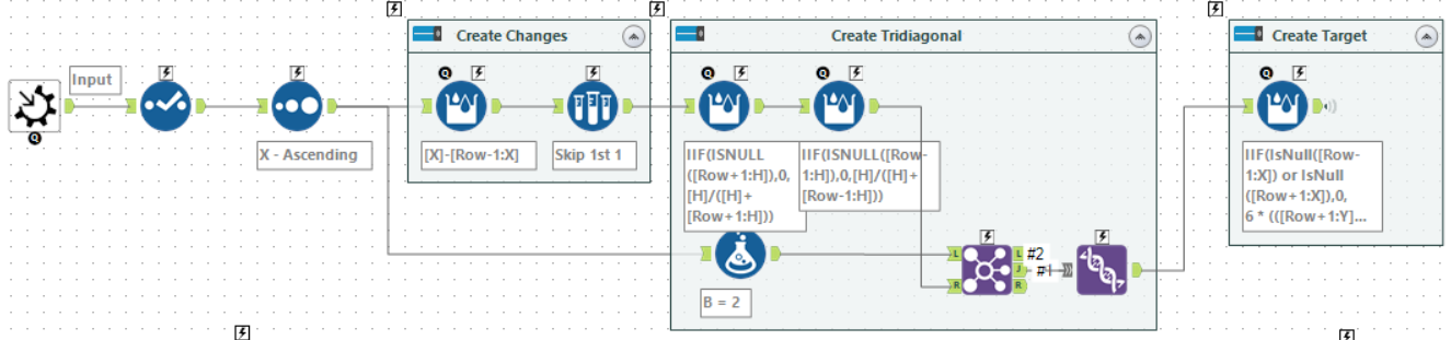
Using some Multi-Row Formula tools it is fairly easy to create these. The expressions are shown below. In all cases the value is a Double and NULL is used for row which don’t exist:

H=[X]-[Row-1:X]
A=IIF(ISNULL([Row+1:H]),0,[H]/([H]+[Row+1:H]))
C=IIF(ISNULL([Row-1:H]),0,[H]/([H]+[Row-1:H]))
B=2

Then using a Join (on row position) and a Union to add the last row to the set. Finally, D is given by:

IIF(IsNull([Row-1:X]) or IsNull([Row+1:X]),
    0,
    6 * (([Row+1:Y]-[Y])/[H] - ([Y]-[Row-1:Y])/[Row-1:H]) / ([H]+[Row-1:H])
)

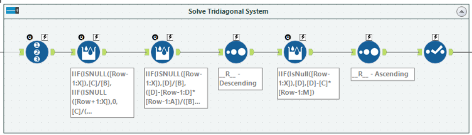
Now to solve the produced system. In order to save on storage, instead of creating C’ and D’, the multi-row formula tools update the values of C and D:

C=IIF(ISNULL([Row-1:X]),[C]/[B],IIF(ISNULL([Row+1:X]),0,[C]/([B]-[Row-1:C]*[Row-1:A])))
D=IIF(ISNULL([Row-1:X]),[D]/[B],([D]-[Row-1:D]*[Row-1:A])/([B]-[Row-1:C]*[Row-1:A]))

To compute the solution vector, M, it is necessary to reverse the direction of the data. While you can use Row+1 to access the next row in a multi-row formula tool, it won’t allow a complete full computation backwards. To do this, add a Record ID and then sort the data on it into descending order. After which M can be calculated using another multi-row formula:

M=IIF(IsNull([Row-1:X]),[D],[D]-[C]*[Row-1:M])

After reverting the sort, we now have all the inputs. So can move to compute the coefficients for each piece of the spline:

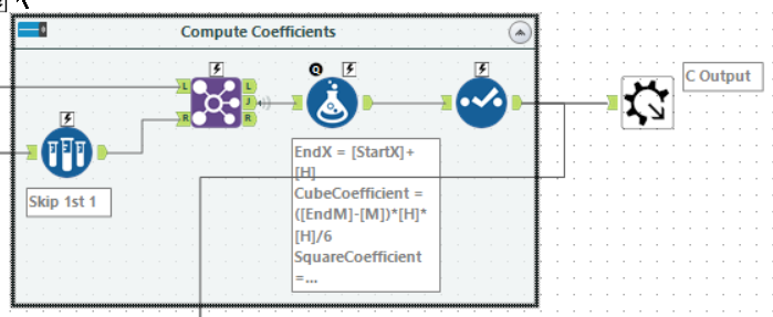
One small trick here is to skip the first row and join back to the same stream. This gives x, y and M for the next row. The coefficients are then computed using a normal formula tool:

CubeCoefficient=([EndM]-[M])*[H]*[H]/6
SquareCoefficient=[M]*[H]*[H]/2
LinearCoefficient=([EndY]-[Y]-([EndM]+2*[M])*[H]*[H]/6)
Constant=[Y]

The final challenge is to reproduce the bisect functionality to find the row for each wanted X.

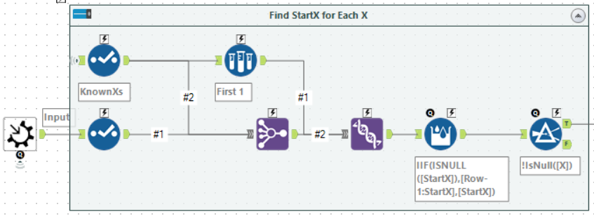
In this case, using a Multiple Join allows creating a full-outer join of known and wanted X values. After this, add the first KnownX at the top and use a multi-row formula to fill in the gaps.

The last step is just to compute the spline. First, join to get the coefficients and then just a standard formula tool to calculate the fitted value.

Having wrapped it up as a macro, a quick test to see it worked:

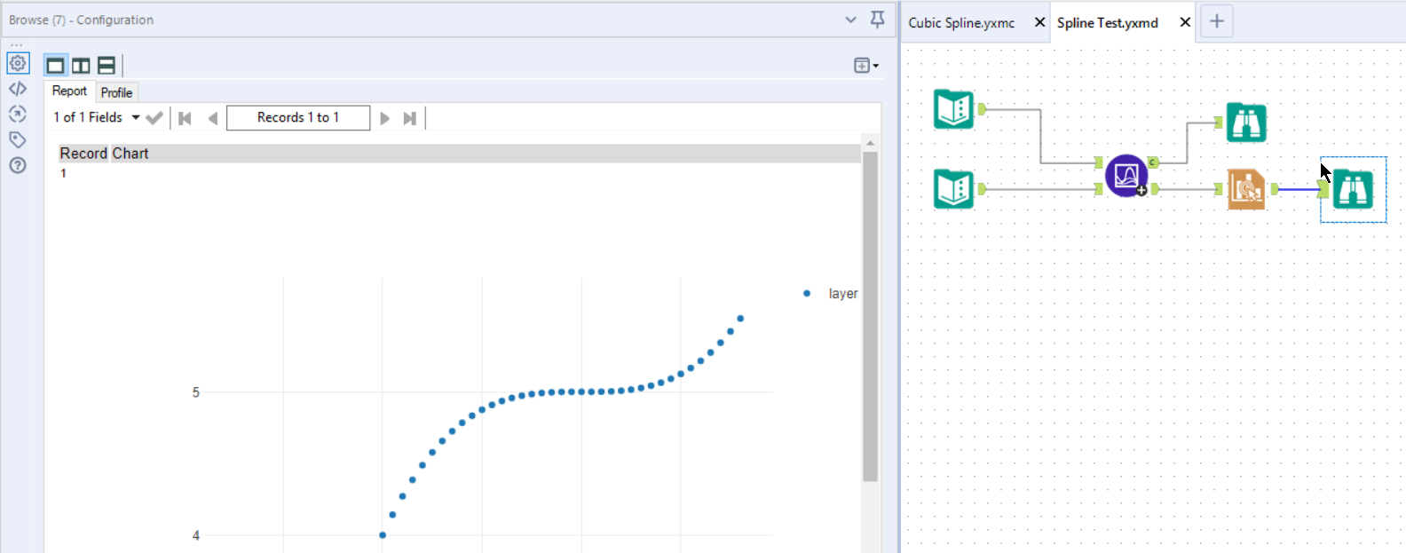
The final macro and test workflow can be downloaded from DropBox (macro, workflow).

Wrapping Up

Hopefully, this gives you some insight into how to build a cubic spline and also how to move some concepts from programming straight into Alteryx.