Trees as a data structure come in various types with a differing number of child nodes. One major component of a tree structure is that it expands in one direction, meaning there are no cycles.

Some popular types of trees are:

Heaps which allows an ordering both as a min heap or a max heap. Pushing the min/max value to the top as the root.

Tries used for character storage. Imagine a spell checker traversing each letter down the tree.

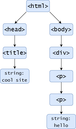
Parsing Trees e.g. HTML tree which allows for the DOM to organise all the elements within the page. With HTML being the root, and head / body being child nodes.

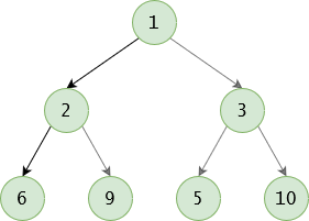
However, today we’ll be looking at the basics around the most popular tree structure, the binary tree. A binary tree gets its name from having a maximum of two nodes. This allows each node to have a left and a right subtree that, in itself, is also a binary tree. For a tree to be classed as complete

Terminology

To help understand trees, and more specifically binary trees, it’s best to get a good understanding of the vocabulary behind them. Below is a list of the most common words used when describing and working with trees.

Root - The node at the very top of the tree.

Leaf - A node with no children.

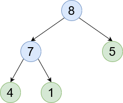
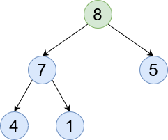
Parent and Children - Nodes below the current node (seen in green) are children. Whereas ones above the current node are parents.

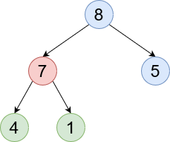
Ancestor - A node somewhere along that branch. 8 is an ancestor of 4.

SubTree - Each node is its own tree. So a child is a subtree of the current tree. Here we can see [7, 4, 1] are a subtree of 8.

Tree State

A tree state is a way to describe the current tree’s setup based on its nodes. It helps identify if a tree is healthy and not too unbalanced.

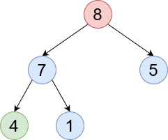
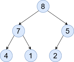
Full - A tree is classed as full if all leaf nodes have no children.

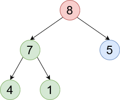
Complete - When a tree is filled in the left-to-right format it is classed as complete. So no lone right leaf nodes without a left one.

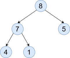
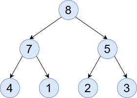
Perfect - All leaves are on the same level with no children and all other nodes have exactly two children.

Traversal

Using a tree is great for storing and accessing the right data. With that there are three ways to traverse a tree. Here we will be exploring that.

Pre Order - (L N R) As the name suggests, pre order is accessing the left node before accessing the current one. This will allow us to explore the entire left branch first and slowly make our way in.

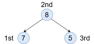
In Order - (L N R) Here we access the node first, then go left and right. This way of accessing is probably the most common. It’s used when creating things like a binary tree search to see which node to go to next or to evaluate if we’ve found our item.

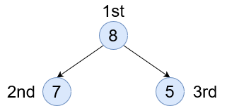
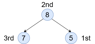
Post Order - (L N R) This is the inverse of the pre order. We access all right nodes first, before accessing the current node.

The Innards

A common choice of tree is a Binary Search Tree (BST). Here we will create one and see how the gubbins work. Firstly we need to create the struct for the node:

struct node{
  int val;
  node* left;
  node* right;
};  

This allows us to build in memory each node and handle it. Next we need to build the constructor to create the root node.

node* create(int val) {
  node* n = new node;
  n->val = val;
  n->left = NULL;
  n->right = NULL;
  return n;
}


BinaryTree(int val){
    root = create(val);
}

We abstract the create method to allow us to build more nodes later and for ease of reading.

The next task is to insert a value into the tree. To give the user a presentable method sigature it’s worth writing a helper method to hide the internal calls within the class.

private:
  void insert(node* n, int val) {
    if (!n) return;
    // Check which side the value should go
    if (n->val <= val) { 
    
      // left block for lower
      if (!n->left) {
        n->left = create(val);
      } else {
        insert(n->left, val);
      }
      
    } else {
      
      // right block for higher
      if (!n->right) {
        n->right = create(val);
      } else {
        insert(n->right, val);
      }
    }
  }

public:
  void addItem(int val) {
    insert(root, val);
  }

Lastly we need to create a nice print method so we can see if the values are actually being stored.

void printTree(node* n) {
  if(n){
  printTree(n->left);
  cout << "  " << n->val << " ";
  printTree(n->right);
  }
}

Put it all together and we have the following:

#include <iostream>

using namespace std;

struct node{
  int val;
  node* left;
  node* right;
};  

class BinaryTree {
  private:
    node* root;
    void insert(node* n, int val) {
      if (!n) return;
      // Check which side the value should go
      if (n->val >= val) { 
        // left block for lower
        if (!n->left) {
          n->left = create(val);
        } else {
          insert(n->left, val);
        }
      } else {
        // right block for higher
        if (!n->right) {
          n->right = create(val);
        } else {
          insert(n->right, val);
        }
      }
    }

    // create and build node for use
    node* create(int val) {
      node* n = new node;
      n->val = val;
      n->left = NULL;
      n->right = NULL;
      return n;
    }

    void printTree(node* n) {
      if(n){
        printTree(n->left);
        cout << "  " << n->val << " ";
        printTree(n->right);
      }
    }


  public:
    BinaryTree(int val){
      root = create(val);
    }

    void addItem(int val) {
      insert(root, val);
    }

    void print() {
      printTree(root);
    }
};

int main() {
  BinaryTree tree = BinaryTree(5);
  tree.addItem(3);
  tree.addItem(7);
  tree.print();
  return 0;
}

Upon running we can see that the output of 3 5 7 shows us that the ordering has taken place. With the knowledge we’ve gained we can say that not only is this tree balanced, but it’s also perfect as 3 and 7 have no children and are at the same level.

The above is a very simple tree that has no node deletion functionality. Have a go and see if you can create your own deletion!