
Recently I’ve been learning about Neural Networks and how they work. In this blog post I write a simple introduction in to some of the core concepts of a basic layered neural network.
What is a neural network made of?
All neural networks are made up of a network of neurons, much like the brain that they model, but what is a neuron?
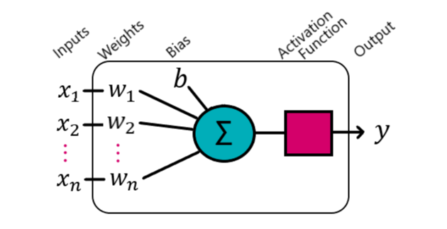
A neuron is made up of its inputs, weights, a bias, an activation function and a singular output. It was originally intended to replicate the biological neuron.
There is a one-to-one ratio of inputs to weights, which when combined gives a series of weighted inputs that get summed together. To this sum a bias gets added.
This can be represented mathematically as follows
\[y = \sum^n_{i=1}w_{i}x_{i}+b\]- \(w\) is the weight
- \(x\) is the input
- \(b\) is the bias
- \(n\) is the number of inputs
Why is an activation function important?
A neuron, with a single input, is a linear function, \(y = ax+b\), and as such can only form simple decision boundaries. An increase in the number of inputs and neurons in the neural network will still result in a linear function. This is because multiple linear functions, when combined, always results in a linear function.
To resolve this issue, and allow the network to find complex decision boundaries, one that wiggles around separating multiple classes, we need to use activation functions, they add non-linearity.
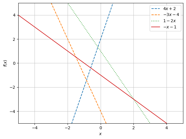
In the following graphs you can see examples of this, the dashed lines represent a neuron with a single weighted input, with the solid red line being the sum of the three. See how in the first graph the red line is still a linear function. Mathematically this is because \((4x + 2) + (-3x - 4) + (-2x + 1)\) simplifies to \((-x - 1)\)
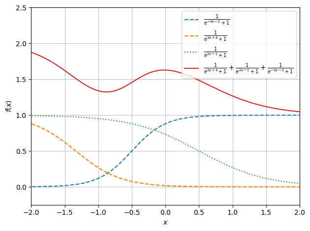
When putting the same neurons through activation functions, in this case logistic functions, non-linearity has been added to the system.
Below are a few of the more known Activation Functions ### Step Function
\[f(x) =\begin{cases}0 & x < 0\\1 & x \geq 0\end{cases}\]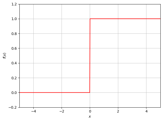
Included for historical reason, this is the original activation function, used in the original perceptron in the 1950’s. This function converts the output of the summation function into a binary value.
Due to the nature of the step in the function, changes to the weights and bias make no difference until the output crosses the step boundary, at which point it flips the binary value.
Logistic Function a.k.a Sigmoid function
\[f(x) = \frac{1}{1 + e^{-x}}\]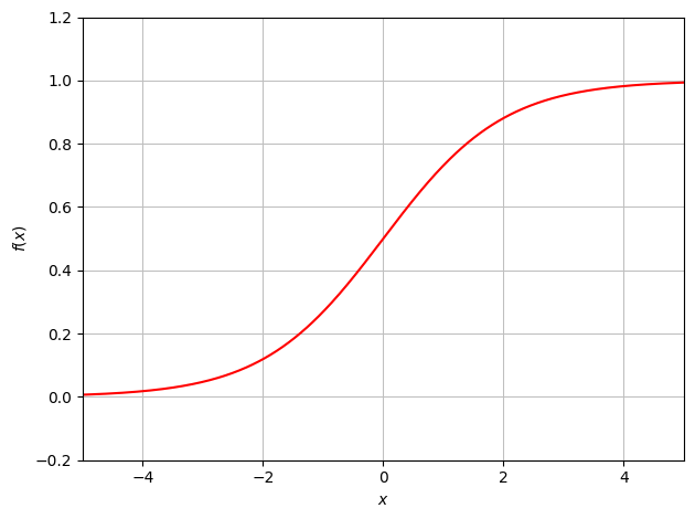
The Logistic function, a variant of the sigmoid function, initially replaced the step function. Like the Step function it limits the output of a neuron between 0 and 1 but doesn’t have the same issues around the zero mark. This makes it easier to train as a change to the weights and biases will always have an effect, except at the extremes.
Rectified Linear Unit (ReLU)
\[f(x) = max(0,x)\]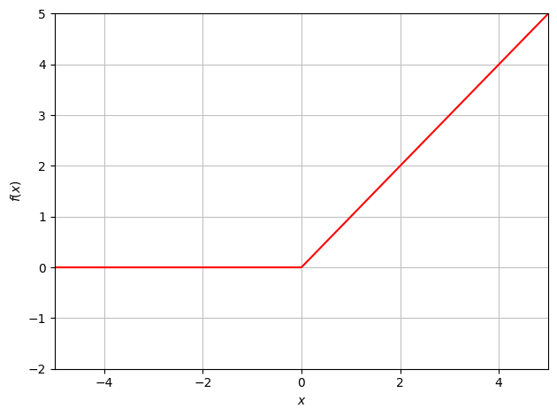
The Rectified Linear Unit (ReLU) has become the most popular and in most cases the default activation function to use for deep neural networks. It takes the maximum value of either 0 or the input, essentially putting any negative input value to 0 immediately.
SoftMax
\[\delta(z) = \frac{e^{z_{i}}}{\sum^{K}_{j=1}{e^{z_{j}}}}\]- \(z\) a vector containing the output values
- \(K\) the number of output values
The SoftMax Activation function is used for the final output layer for classification neural networks. It converts a vector of the output values into a probability distribution over the output classes. Each output neuron will then represent the probability the input is of the respective class.
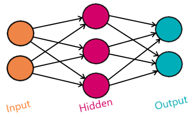
Architecture of a Neural Network
In neural networks, the neurons can be arranged in a variety of ways. For the basic neural network the neurons are arranged into several distinct layers.
There are three categories
- Input Layer
- Hidden Layers
- Output Layer
1. Input Layer
The input layer is purely the values of the input data, no calculations take place. There is a neuron for each input value, for image classification neural networks of grey scale images there would be a neuron for each pixel.
2. Hidden Layers
The hidden layers are the work horse of the neural network, they are responsible for identifying features or transforming inputs into something the output layer can use.
If there is a single hidden layer, then the neural network is a shallow neural network. If there are two or more hidden layers, then it is a deep learning neural network. The deeper the neural network the more complex patterns the neural network can learn, though this comes at a cost of requiring more computational power to train.
There can be any number of neurons in each hidden layer, the more you have can lead to an increase in the information the neural network can identify in the input. Though an increase in neuron number can lead to over fitting to the training data
3. Output Layer
The output layer gives the output of the neural network. For image classification there would be a neuron for each class of item to be classified, for example in handwritten digit recognition there would be 10 neurons, one for each of the 10 digits.
How the layers are connected
For the basic layered neural network, each neuron takes the outputs of every neuron in the previous layer as its input. With the first hidden layer taking the inputs to the neural network directly.
It has been proven that a neural network which has two layers and uses non-linear activation functions can be a universal function approximator, that can find any mathematical function.
Determining the weights and biases (the parameters)
So how do the weights and biases of each neuron get set?
The weights and biases, the parameters, could be manually updated until the output of the neural network is correct. However neural networks can consist of millions/billions of parameters, so an automated process is needed.
To be able to automate the process, a way of evaluating the accuracy of the neural network is needed. To do this a loss function can be used to give a value that shows how far away the current neural network is from making a correct evaluation.
Loss Function
A common algorithm for finding the error of the neural network is the Mean Squared Error function. This finds a positive value showing how far from the expected value the network is.
\[MSE = \frac{1}{n}\sum_{i=1}^{n}(Y_{i}-Ŷ_{i})^{2}\]- \(Ŷ\) is the actual network output
- \(Y\) is the expected value of class
- \(n\) is the total number of output neurons.
The loss function enables an empirical analysis to see if the change in parameters improves or worsens the output of the neural network. The goal is to change the parameters to minimise the loss as much as possible.
A method called Gradient Descent can be used to determine how to adjust the parameters to reduce the loss.
Gradient Descent
Assume a single input neural network, with a single weight. If we plotted the weight v loss graph, we could have something like the following graph.
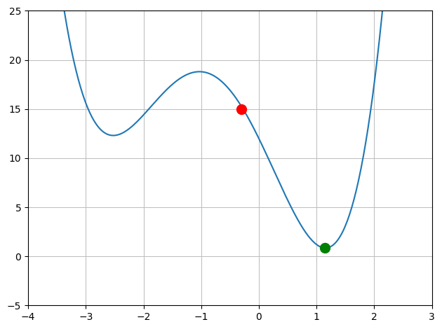
Say the red marker is the current value of the error based on the current weight and the green dot is the minimum error. The aim is to calculate the value of weight that gives us that minimum value.
To calculate the new weight value, take the derivative of the error in respect to the weight and subtract the value from the current weight. In effect finding a new value that is lower down the slope of the graph towards the local or global minima.
\[w_{i+1} = w_i - \alpha\frac{\delta L}{\delta w_i}\]- \(w_{i+1}\) is the new weight
- \(w_i\) the current weight
- \(\alpha\) the learning rate
- \(\frac{\delta L}{\delta w_i}\) is the derivative of the change in loss against weight
The learning rate is used to control how much of a change to the weight is made, if the size of the weight change is too big then loss minima may be stepped over or it may never settle in the “valley” of the minima and constantly jump from side to side. If it’s too small, then it will take longer to reach the local minima.
Back Propagation
To calculate the adjustment for every weight, then the gradient of the change in error with respect to change in each weight needs to be calculated. To do this for the final layer is simple, but for earlier layers it’s not so simple.
A mathematical concept called Back Propagation can be used to determine this, where starting at the last layer, the derivatives are calculated layer by layer toward the first layer.
A calculus concept called Chain Rule is used as part of the back propagation to calculate the gradient of the error function with respect to each layer’s inputs, weights and biases.
Back Propagation is complex so to learn more about it and how it works the fantastic youtube channel 3 blue 1 brown explains it here.
Conclusion
In conclusion, this blog covered the core concepts of Neural Networks, giving an overview on their functionality and learning mechanisms. I hope this brief delve into the architecture and mathematics behind the neural network has given you a good first glance into the world of Neural Networks and inspired you to delve deeper into this fascinating subject.